Zhewei Sun

Baseline Results

Here we present the results of the baseline tests in default mode. The default mode of the program includes all baseline features described in the specification, plus a subset of the extra features implemented. The following results are obtained using 24x24 feature descriptors with GLOH and two-sided ratio test with kd-tree.

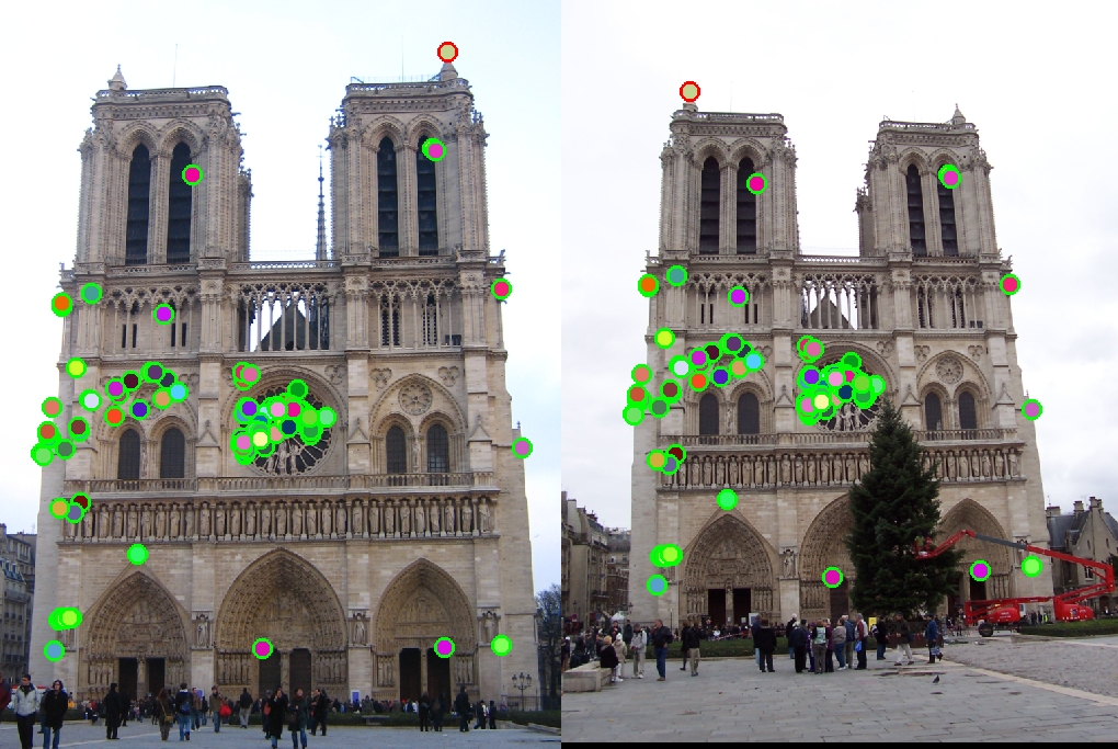
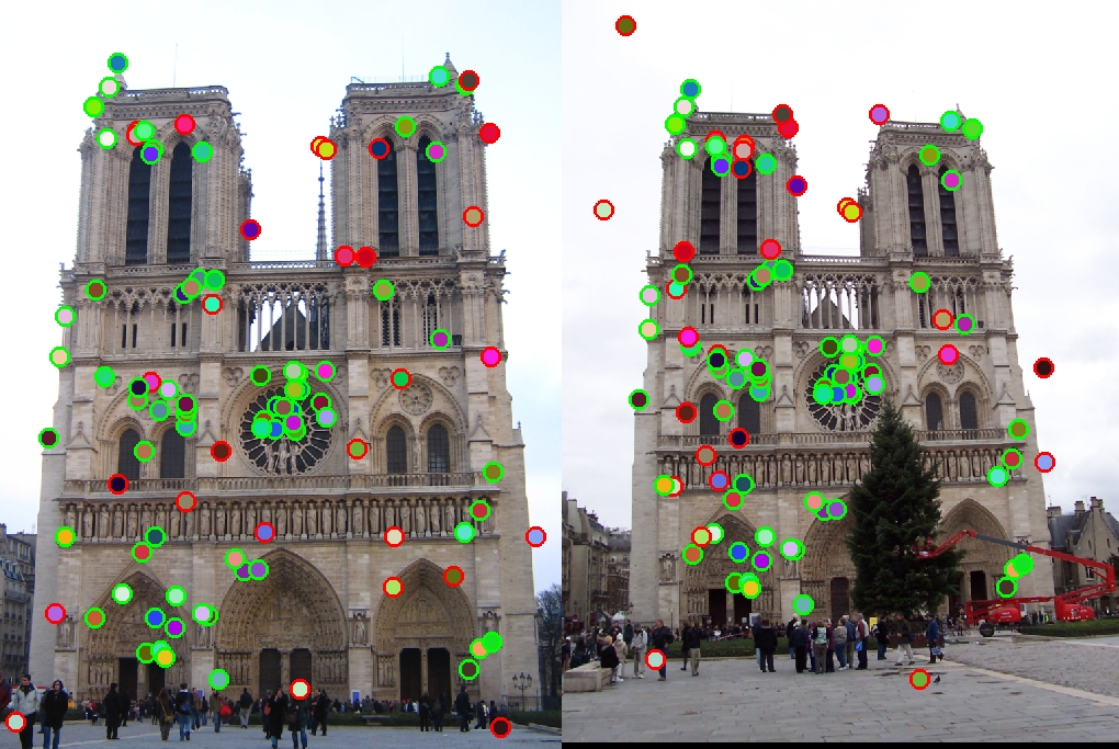
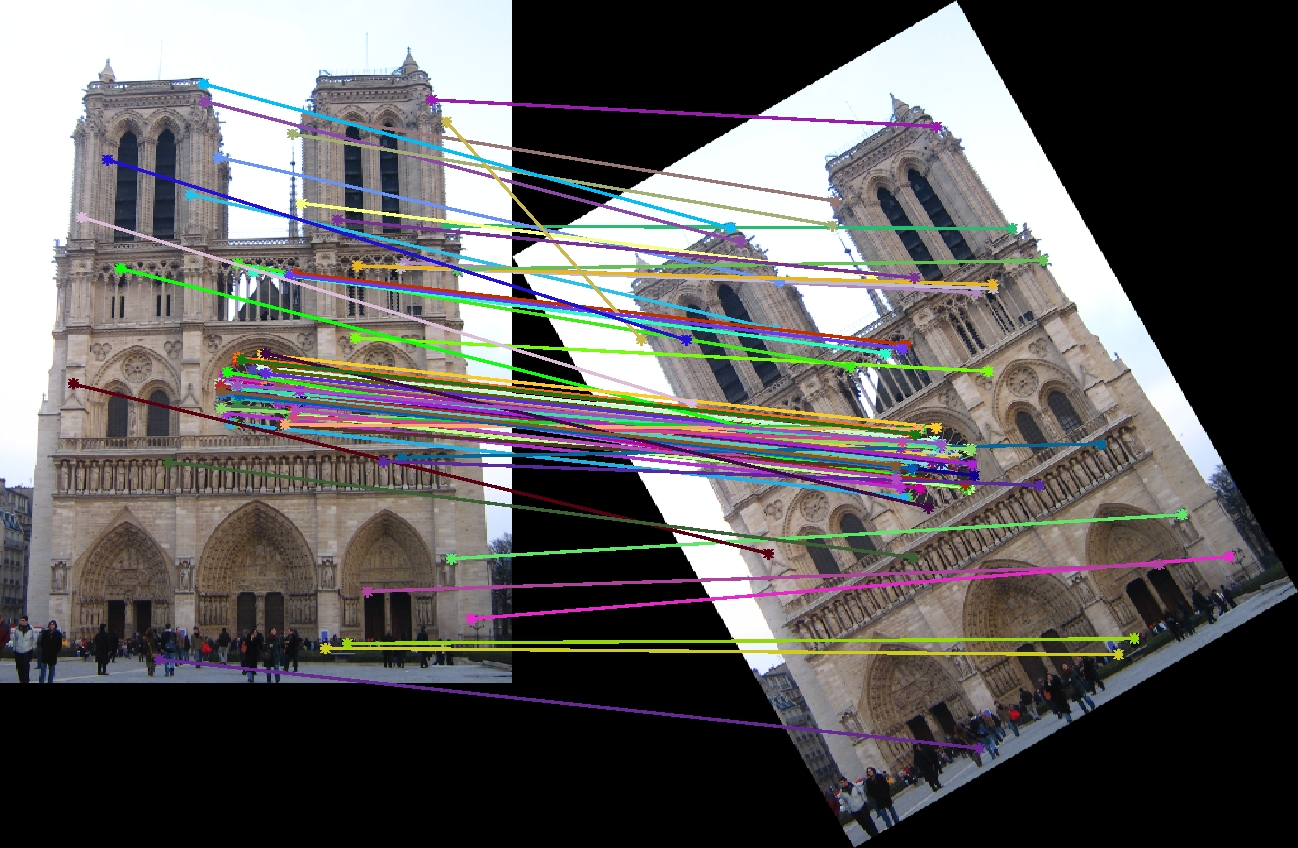
Notre Dame Baseline Result - Accuracy: 99%

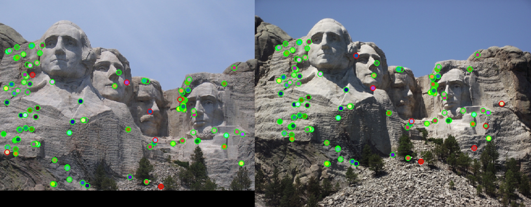
Mount Rushmore Baseline Result - Accuracy: 93%

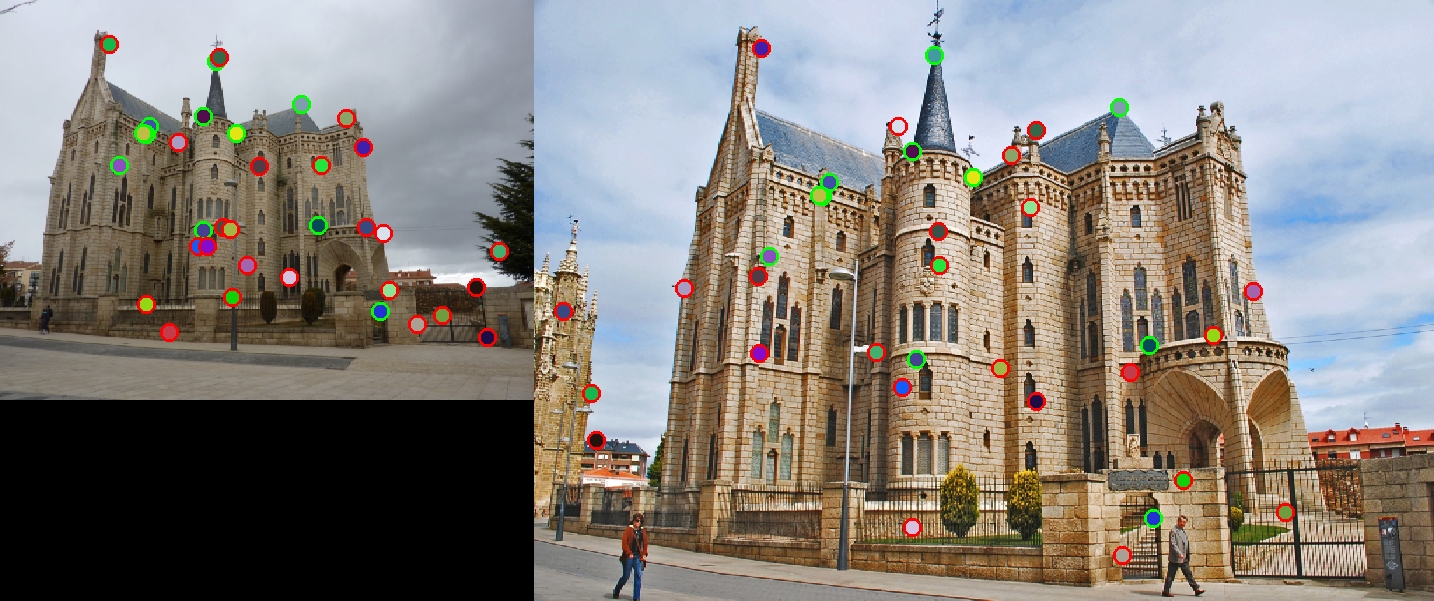
Episcopal Gaudi Baseline Result - Accuracy: 31% - 35 Total Matches

As shown above, the Notre Dame and Mount Rushmore test cases perform quite well with very high accuracy. The Episcopal Gaudi case does not perform nearly as well because of the different scales. To show this, we present some alternative sets of Episcopal Gaudi images below with similar scales.

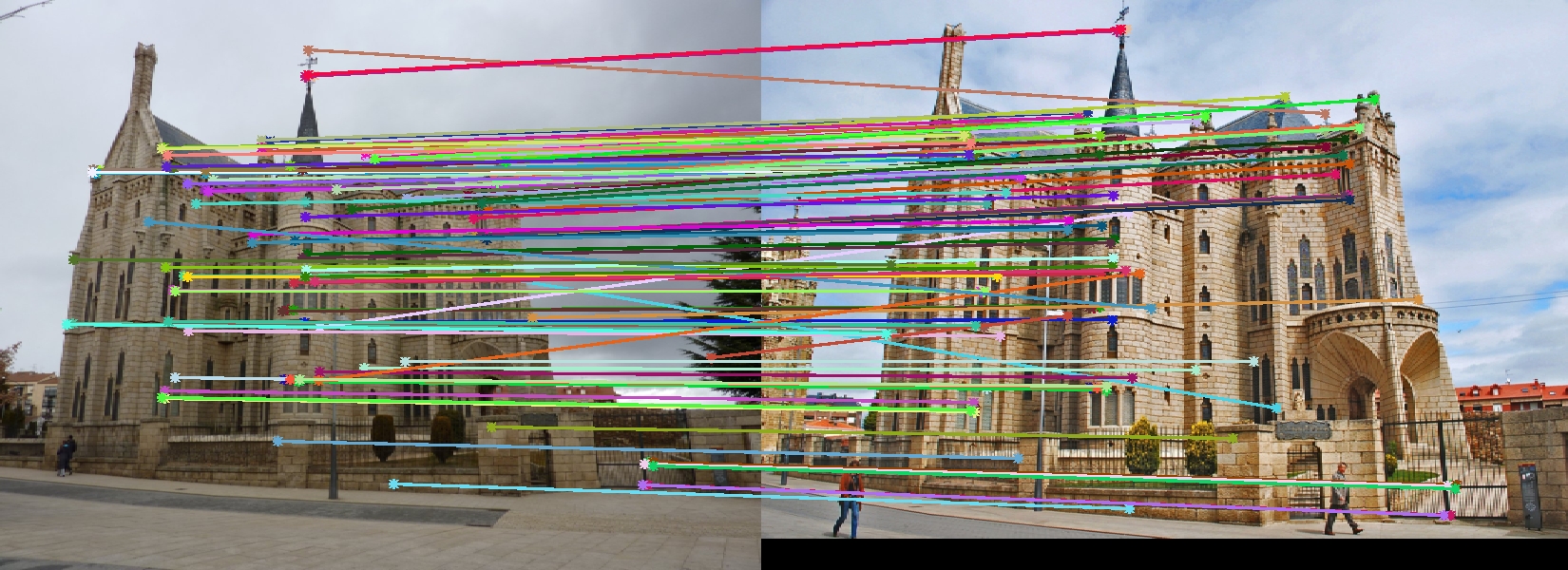
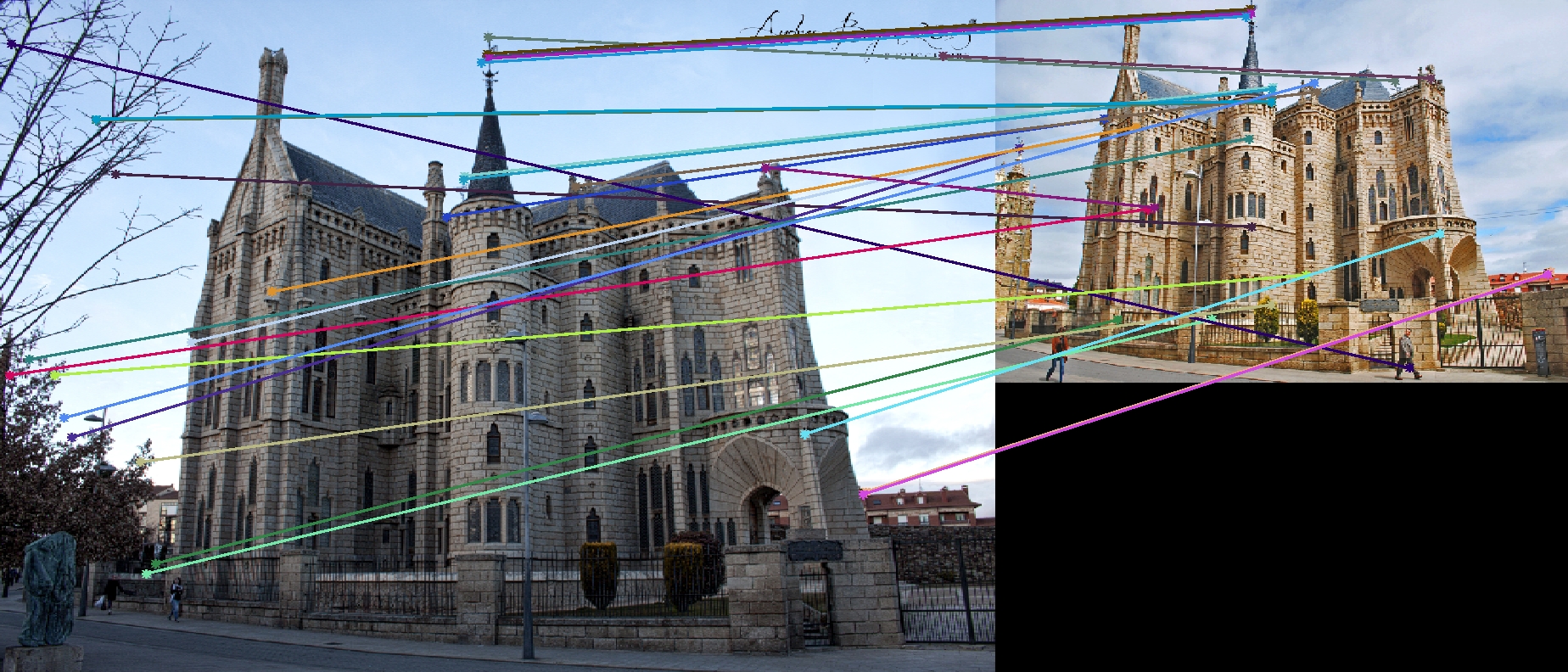
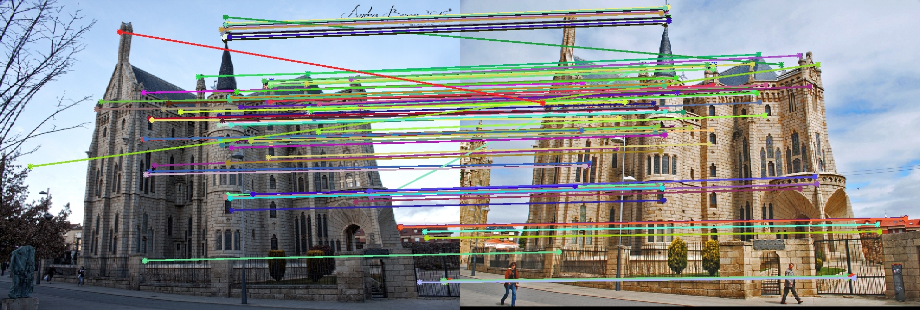
It is clear that the algorithm performs much better when the images are closely scaled. Therefore, the lack of scale invariance in the pipeline have caused poor performance on the Episcopal Gaudi set.

Implementation Highlights and Results

Here we present the implementation details of the project including many bells & whistles. We also show the results of the extra features implemented.

Interest Point Detection

Interest points are found by first computing the Harris cornerness score on each pixel of the image. Then we remove all scores below a certain threshold. Finally, non-maximal suppression is used to remove points that are not local maximums. We use the remaining set of points (up to a certain upper limit, 4000 in default) as our interest points. In the default implementation, the non-maximal suppression is implemented by calling max on a 3x3 sliding window for each pixel. This approach happens to work better than the connected components approach where it increased the accuracy by 5%.

The detector can also estimate the orientation of an interest point, which is useful in situations where the two images undergo a significant rotational transformation. The orientation is estimated by using a 36-bin histogram of gradient directions, where each pixel in an 8x8 window casts a weighted vote (by gradient magnitude) on its respective direction. Then we select the histogram bin with the highest votes and calculates a weighted average of the gradient directions within that bin. The result is then used as the orientation estimate of the interest point. Relevent results will be shown in the next section when we discuss rotation invariant feature descriptor.

Adaptive non-maximum suppression was also implemented in hope to produce matches that are spatially spread out. The goal is to find a number of goal points (4000 in default) such that any two points in the set are at least distance r apart. We use an iterative approach where we increase the minimum distance r until we cannot find enough points matching the criteria. In each iteration, we first threshold points and then sort them based on their cornerness scores in descending order. Then we iterate through the ordered list and add point to the interest point set if it is at least distance r apart from every other previously found interest point in the set. As a result, we find a set of points with pairwise distance less r that has the highest overall Harris score. In this implementation, r is initially set to 2 and increments by 4 each iteration.

Notre Dame Test Set with ANMS - Accuracy: 71%

As shown above, ANMS is able to find interest points that are more spread apart. However, it comes at a cost of matching accuracy.

Building Feature Descriptors

The feature descriptor builds a 128 dimensional feature vector for each interest points. It does so by first cutting out an image patch of a specified size. Then it calculates the gradients of the pixels within the patch, where each pixel votes a 8-bin gradient direction histogram. The image patch is divided into 4x4 cells and each cell contains a gradient histogram. The histograms are then normalized to construct the feature vector.

The size of the feature patch can have a significant effect on the overall accuracy. The table below shows the accuracy of the baseline tests using different patch sizes. In general, as we increase the size of the patch, the accuracy also increases. The number of matched found however, decreases when we increase the patch size. Hence a default patch size of 24 is used in this implementation.

Test Case \ Patch Size	8	16	24	32
Notre Dame	69%	96%	99%	96%
Mount Rushmore	24%	93%	93%	99%
Episcopal Gaudi	5%	13%	31%	56%

The feature descriptor can be rotation invariant by taking advantage of the orientation estimates the interest point detector provided. It does so by generating a rotated image patch based on the orientation angle given. In this particular implementation, the rotated image patch is generated by computing the pre-transform pixel location for each pixel in the rotated patch. Then it samples the original image using bilinear interpolation to obtain the pixel value. An example of the rotated image patch is shown below:

A feature patch showing the tip of Notre Dame, where the patch on the right was rotated by 160 degrees.

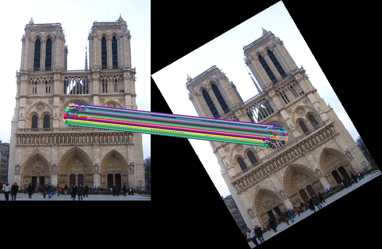
The above two images shows the result of match between a rotated set of Notre Dame without and with orientation estimate/descriptor respectively. In the default baseline result, it is only able to find matches in the center area, where the image is rotationally symmetric. With a rotation invariant feature descriptor, the program was able to find more interesting matches in other regions of the image.

The feature descriptor also implements the GLOH feature - a different binning technique that uses polar distribution instead of a grid distribution. To keep all the testing consistent, our GLOH feature is also 128 dimensional, where the image patch is divided into 8 equal slices based on the angle and each slice is divided into 2 cells by half of the feature width. If the distance between a pixel and the center is greater than the feature width, then we don't consider that pixel. This allows us to not give preference to certain cells. In terms of performance, it gives very similar results when compared to a grid feature, but GLOH seems to be more stable in general. In particular, it gives much better performance on the Episcopal Gaudi set.

Once a feature vector is constructed, the descriptor uses a normalize - threshold - raise power - normalize scheme. This extra normalization step does help and raised the accuracy by a few percent.

Feature Matching

To match feature descriptors built from two images, the nearest neighbour ratio test is used. Each feature descriptor finds its two nearest neighbours, checks the ratio of distances between them, and matches the point with its nearest neighbour only if the ratio is lower than a certain threshold. The ratio test is more robust than simple nearest neighbour matching because it allows us to prune out the ambiguous cases.

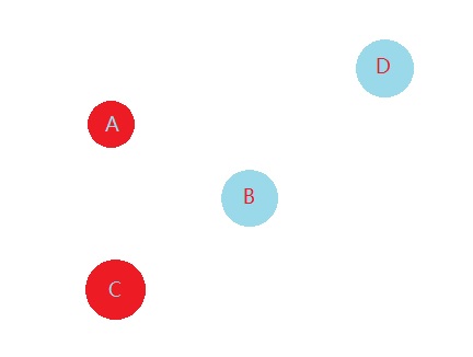
In this implementation, a two-sided ratio test is used. Instead of only one point having to check the ratio against its nearest and second nearest neighbour, we require its nearest neighbour to also pass the ratio test against our original point as its nearest neighbour. To see why this can be helpful, consider the case shown in the figure on the right. In this case, a one-sided ratio test would match point A to point B because |AB|/|AD| is sufficiently small. For point B however, the situation is ambiguous because point A and point C are of the same distance to B. Hence by checking the ratio test from both sides, we can eliminate many potentially bad matches. The table below shows the improvement this match scheme brings to an earlier version of the implementation.

	One Sided	Two Sided
Notre Dame	75%	91%
Mount Rushmore	51%	69%
Episcopal Gaudi	10%	25%

The naive implementation of the nearest neighbour check can be quite slow, thus this implementation uses Matlab's knnsearch function where a kd-tree is built underneath. A kd-tree is useful in this case as its space partitioning properties would allow faster queries. For approximately 4500 feature descriptors in both images, the naive implementation took 33.59 seconds whereas the kd-tree nearest neighbour solver reduced that to 2.27 seconds.

List of Bells & Whistles mentioned in this report

- Keypoint Orientation Estimation

- Adaptive Non-Maximum Suppression

- SIFT Parameter Tuning

- Rotation Invariant Feature Descriptor

- GLOH feature

- Feature Matching using kd-trees