Project 3: Camera Calibration and Fundamental Matrix Estimation with RANSAC
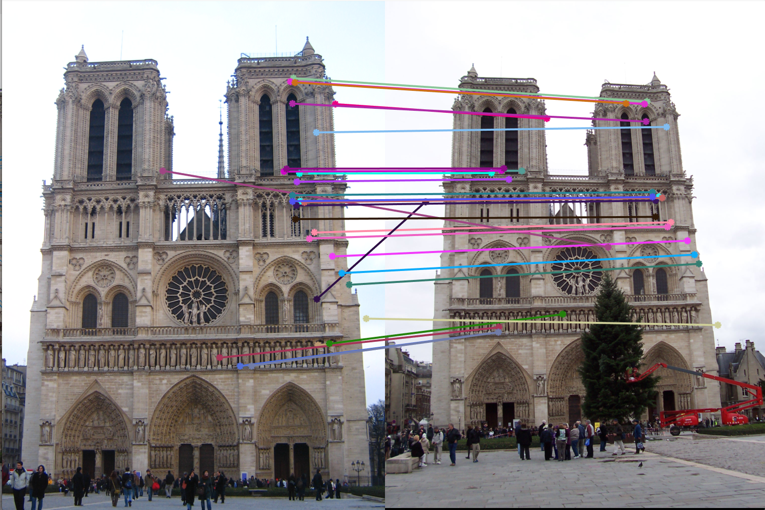
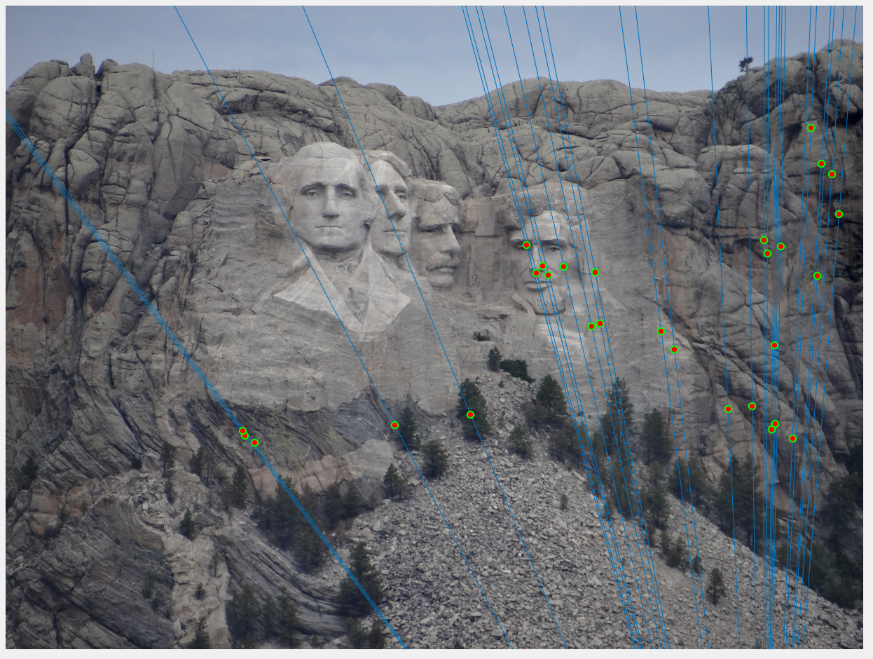
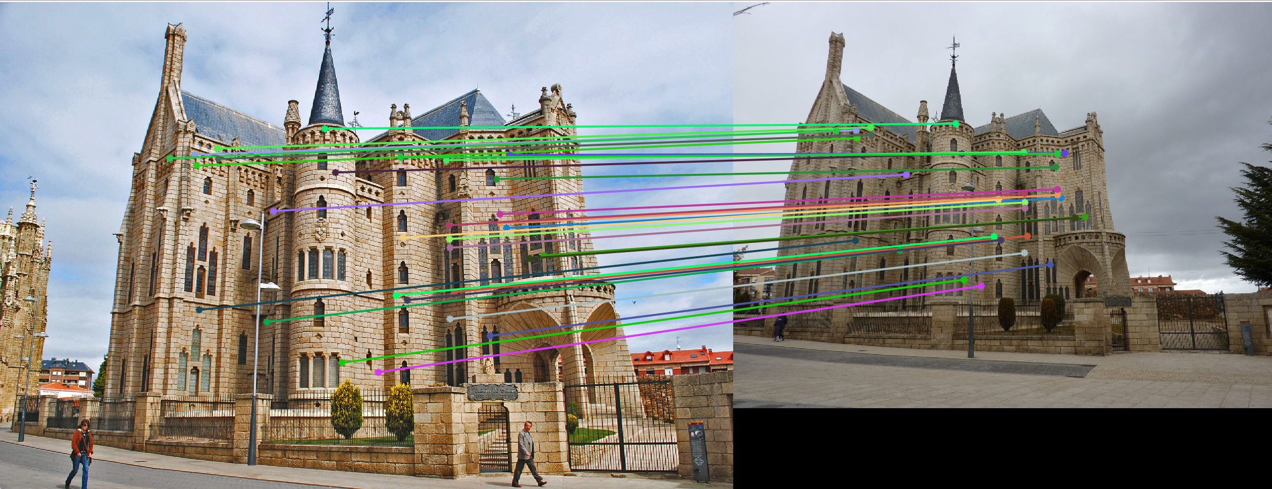
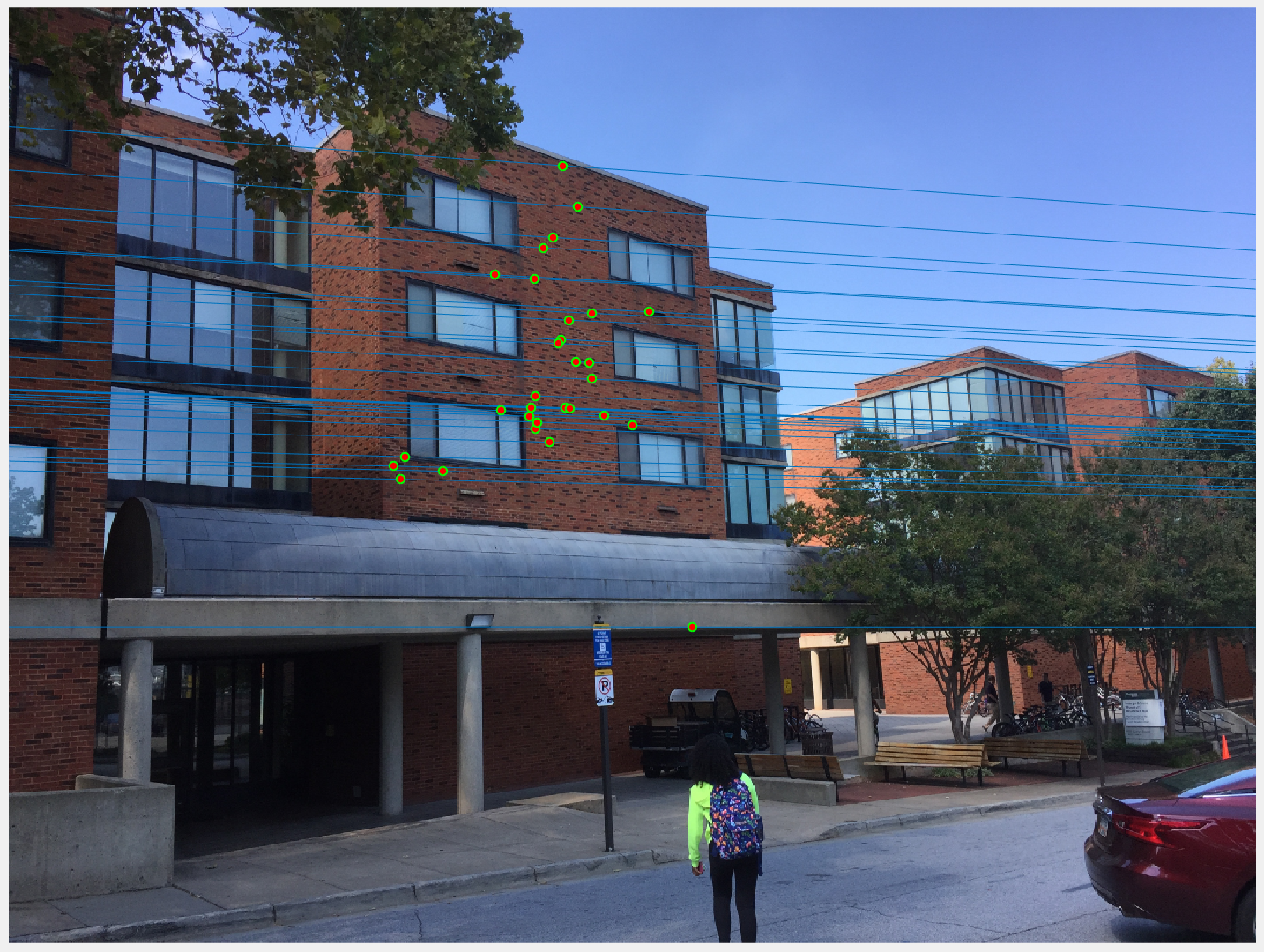
Identification and matching of two images is done by identifying corner points, and matching the features around these corner points. Algorithms like SIFT depend on gradient of image around corner points, and are sensitive to extrinsic parameters such as camera calibration. Thus, if the camera is rotated, or the same object is captured from a different angle as shown in figure 1, SIFT gives very poor results as we saw in project 2.
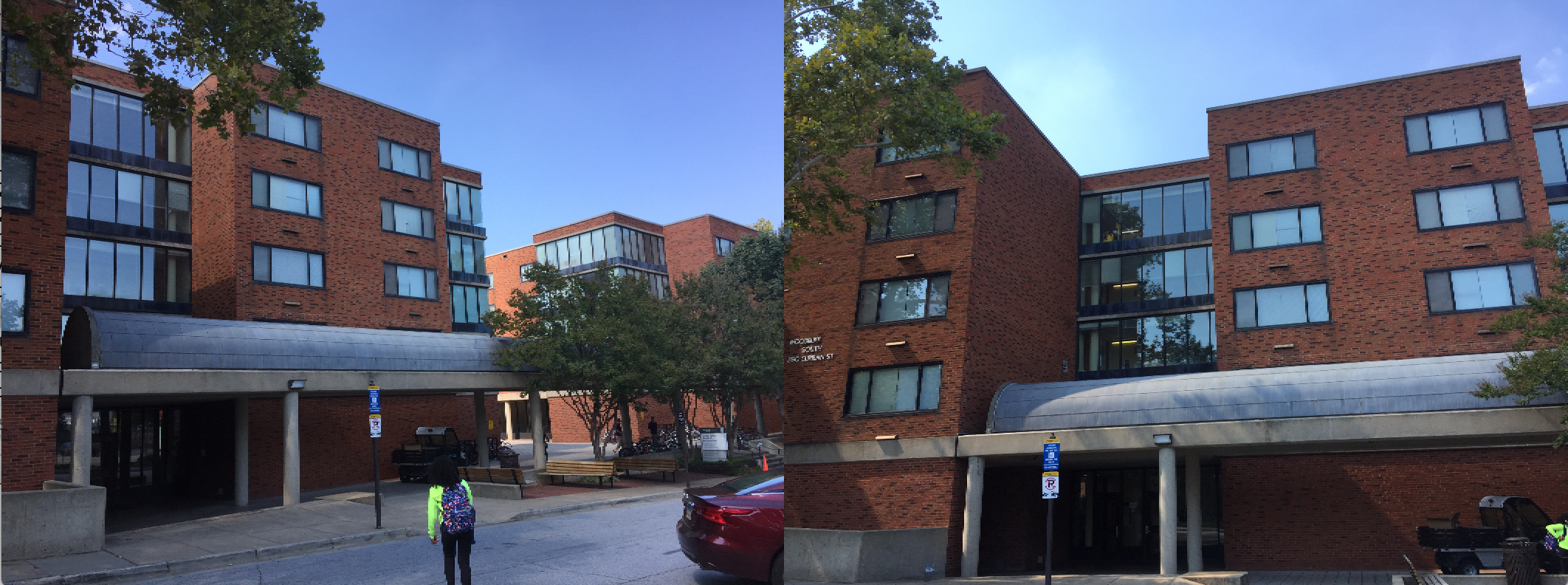
Figure 1: Images of the same building taken at different camera orientations.
Thus, in this project we take into account camera calibration and extrinsic properties such as optical centre, aspect ratio, and skew between x and y axis. The project is devided into three basic components.
- Estimation of Camera Projection Matrix.
- Estimation of Fundamental Matrix.
- Using RANSAC to find Best Estimate of Fundamental Matrix.
EXTRA We first estimate the projection matrix for transforming from real world 3D coordinates to 2D image coordinates by using linear regression. We also estimate the fundamental matrix for transformation from image A to image B taken using different extrinsic properties such as camera roattion etc. Here we use RANSAC to randomly sample points to
I. Estimation of Camera Projection Matrix
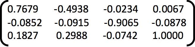
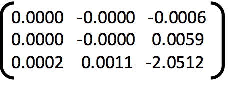
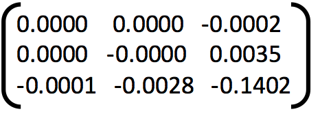
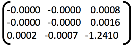
The projection matirix is used to convert from 3D read world coordintes to 2D image coordinates. The structure of this projection matrix is shown in figure 2. We use linear regression to estimate the elements of the 3x4 matrix generated as a product of intrinsic and extrinsic properties of the image.
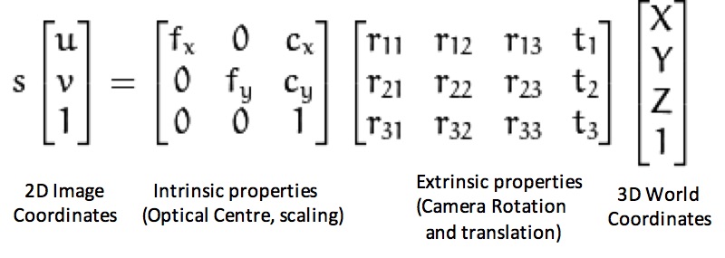
Figure 2: Projection matrix.
In figure 3 we show the actual 2D points and the points obtained from applying the projection matrix on corresponding 3D points. We see that the points overlap, showing that the projection matrix gives a good projection from 3D world coordinates to 2D image coordinates.
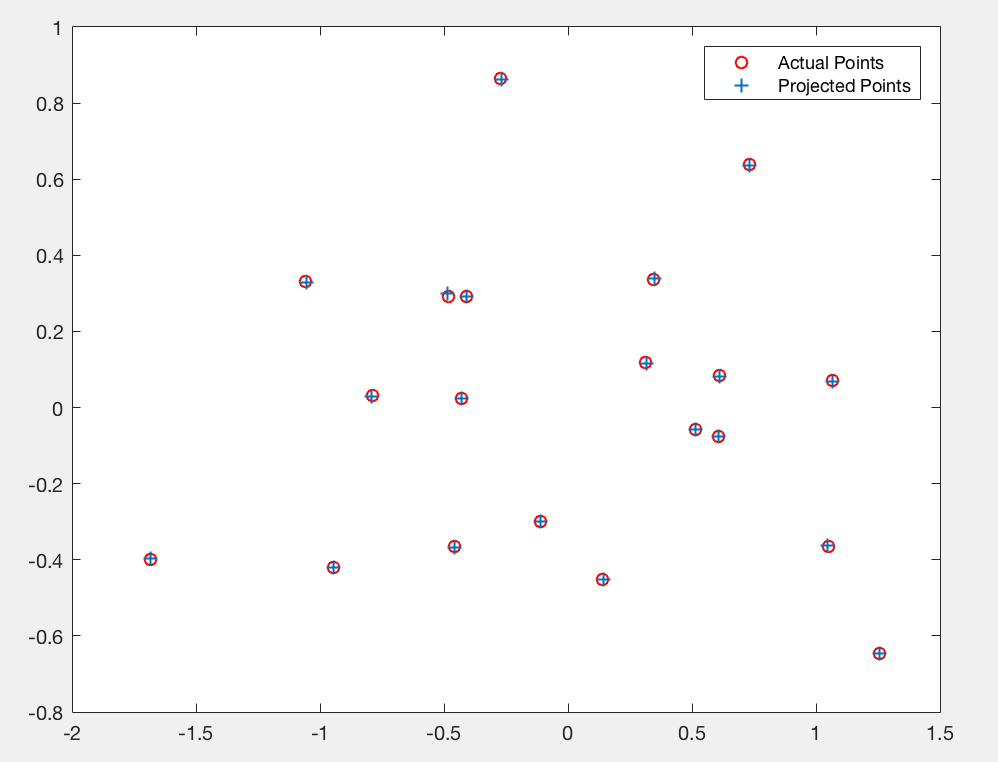
Figure 3: Plot of actual and estimated image coordinates using projection matrix.
Additionally, we also estimate the camera centre (optical centre) from this projection matrix. This done using equations shown below in equation 1 and 2. In figure 4, we can see the camera coordinate in the 3D plot. This gives us a visual description of where the camera is placed with respect to the corner points of the view.
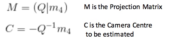
Equation 1: Calculating Camera centre from projection matrix.
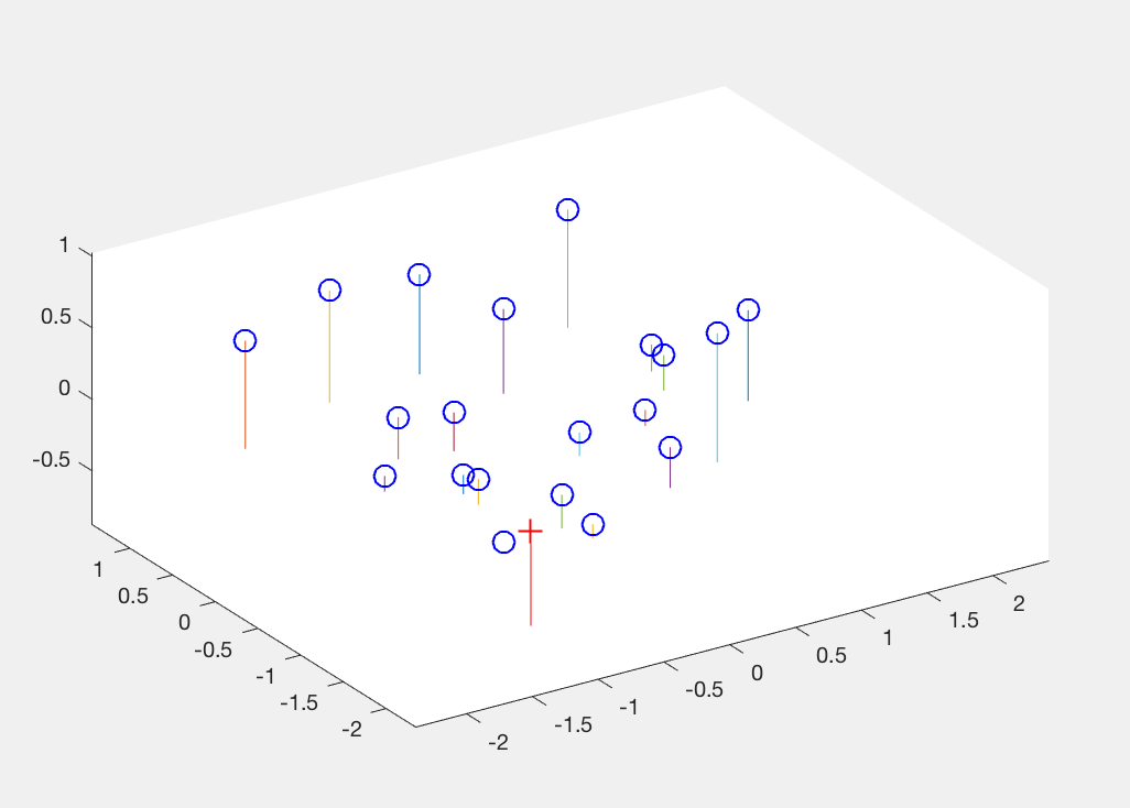
Figure 4: Visual description of Camera centre with respect to interest points in 3D coordinates.
'+' shows the camera centre, 'o' are the interest points.
The above plots have been obtained by using normalized images. Normalized images are mean centred, and have unit variance. Normalized image coordinates have a maximum of unit distance between each other. As a result, the projection matrix gives image coordinates that are closer to the ground truth normalized coordinates. We us Residue as a measure of performance. Residue is calculated as the mean square distance between the projected points obtained using our projection matrix, and the ground truth 2D points. For both the normalized and non-normalized images, we obtain the following residues.
In the case of normalized image coordinates, residue = 0.0445
In case of non-normalized image coordinates, residue = 15.6217.
As we can see, normalization reduces the mean square error of obtained results by a significant factor. In Figure 5, we see the projected points using non-normalized image coordinates, and in fogure 6, we see the camera centre using non-normalized image coordinates.
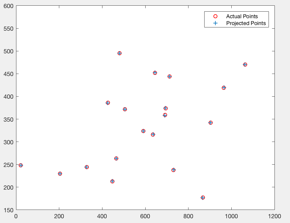
Figure 5: Plot of actual and estimated image non-normalized coordinates using projection matrix.
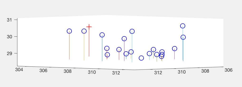
Figure 6: Visual description of Camera centre with respect to interest points in non-normalized 3D coordinates.
'+' shows the camera centre, 'o' are the interest points.
Results:
1. Normalized image coordinates:
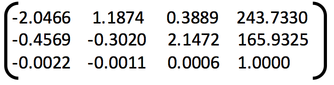
Projection Matrix =
Camera Centre = [-1.5126, -2.3517, 0.2827]
The total residual is: 0.0445
2. Non-Normalized image coordinates:
Projection Matrix =
Camera Centre = [303.0967, 307.1842, 30.4223]
The total residual is: 15.6217
II. Estimation of Fundamental Matrix
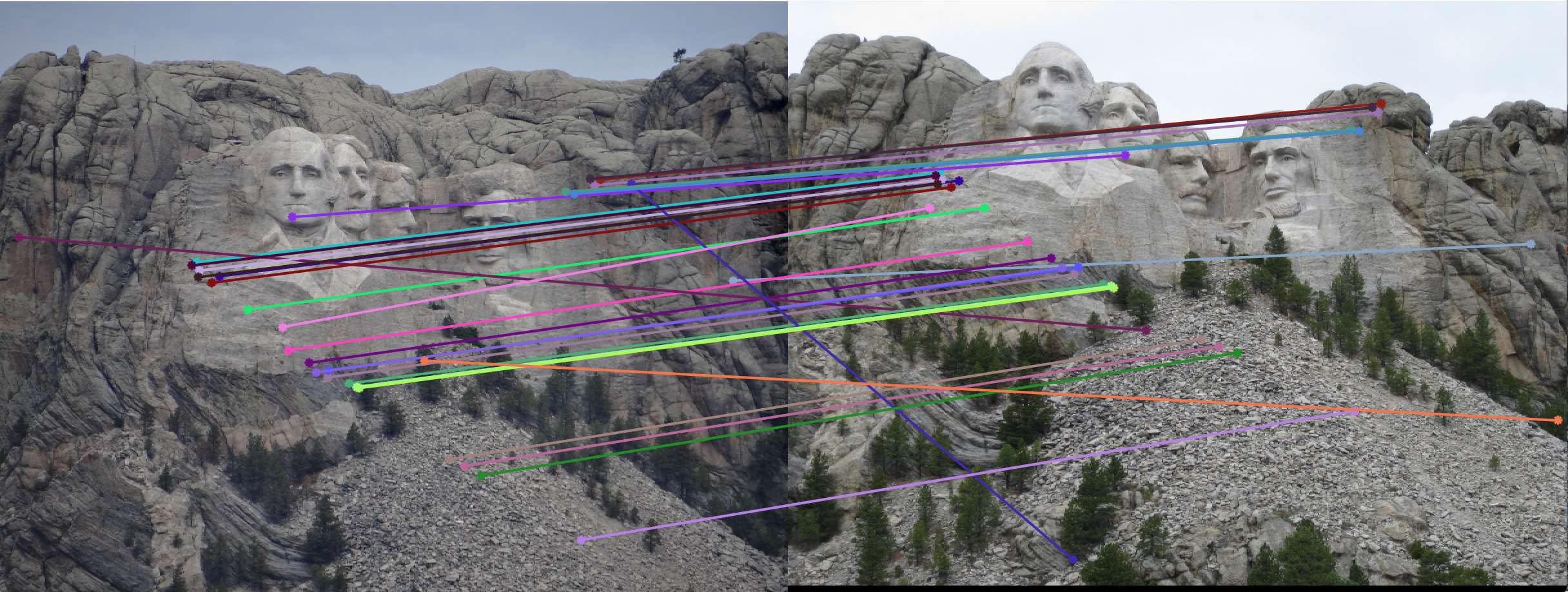
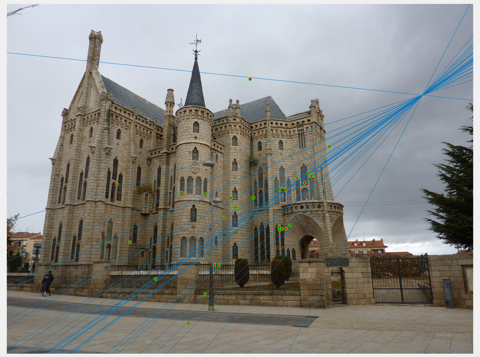
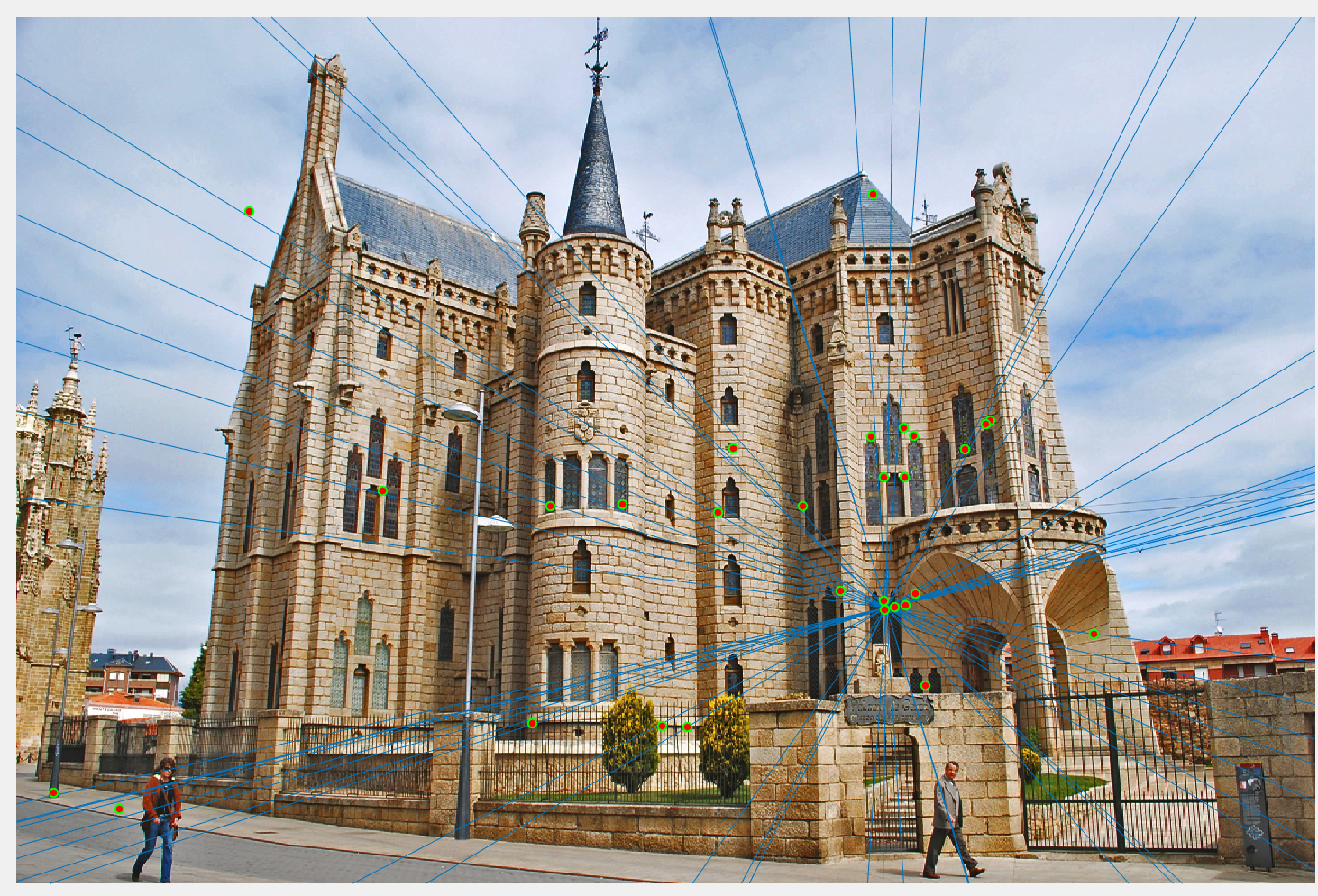
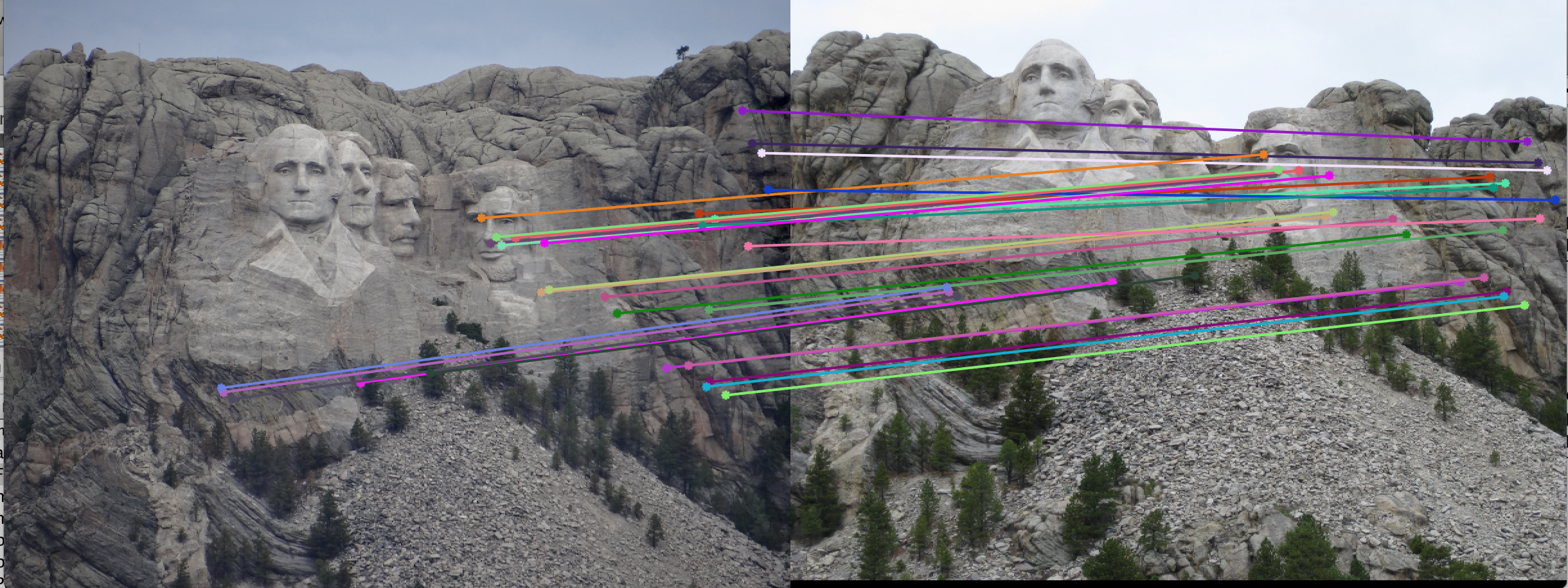
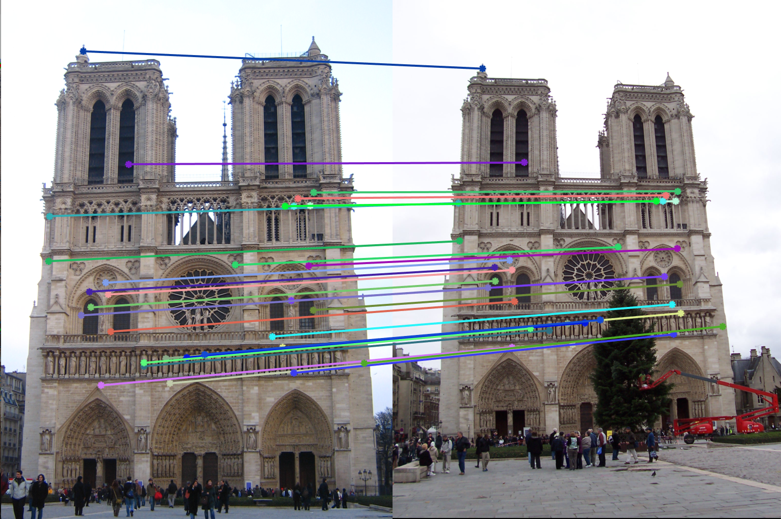
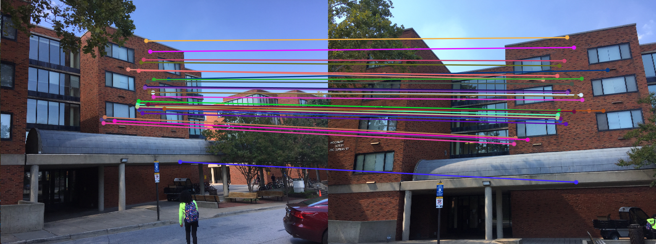
When we have two images with different intrinsic and extrinsic properties, the same point or corner on both the images will have different features. Thus basic SIFT will result is large number of mismatches. THis can be seen in figure 7.
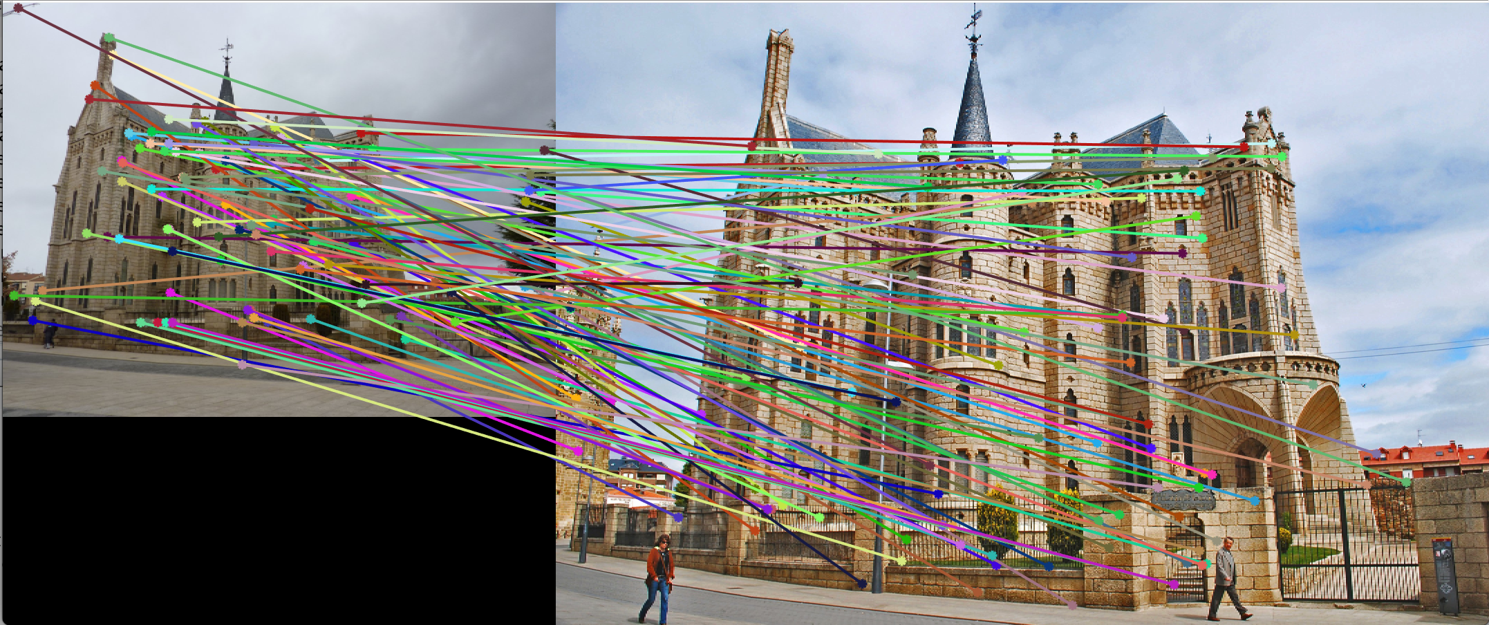
Figure 7: SIFT matches for two images taken with different projection matrices. SIFT gives us poor results for this.
When we have to match two images with different projection matrices, we find its fundamental matrix. The Fundamental martix is constructed using translation and rotation matrix components of camera's extrinsic parameters. The fundamental matrix is deduced as shown in equation 2 below.
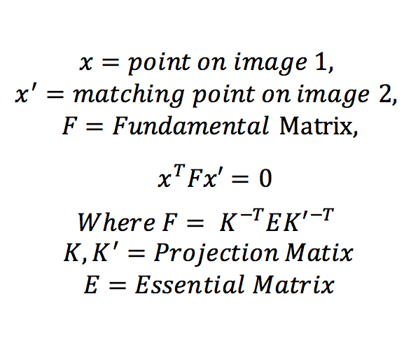
Equation 2: Fundamental Matrix equation.
Fundamental matrix uses the concept of Epipolar Geometry which says that a point in an image can be present only in the corresponding image's epipolar line. Epipolar lines are the lines drawn from a point in 3D world coordinates to the respective image's optical centers. Thus, we estimate the Fundamental matrix as a set of homogeneous linear equations using the 8-point algorithm as shown in equations 3.
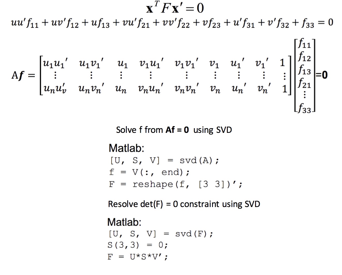
Equation 3: 8-point algorithm
Here, we have obtained the fundamental matrix using two methods.
- Without normalized interest points.
- With Normalized interest points.
1. Fundamental Matrix estimation WITHOUT normalization:
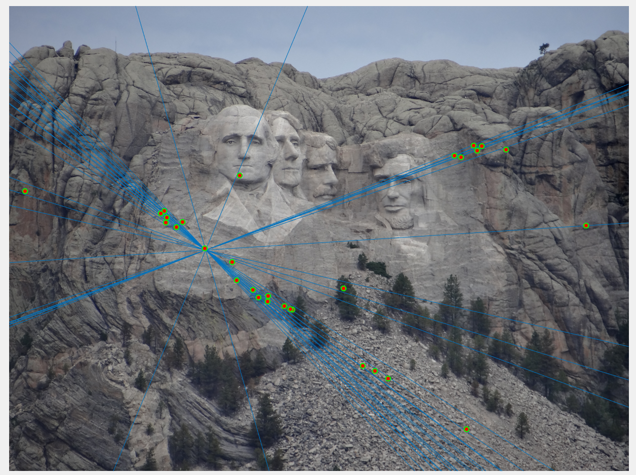
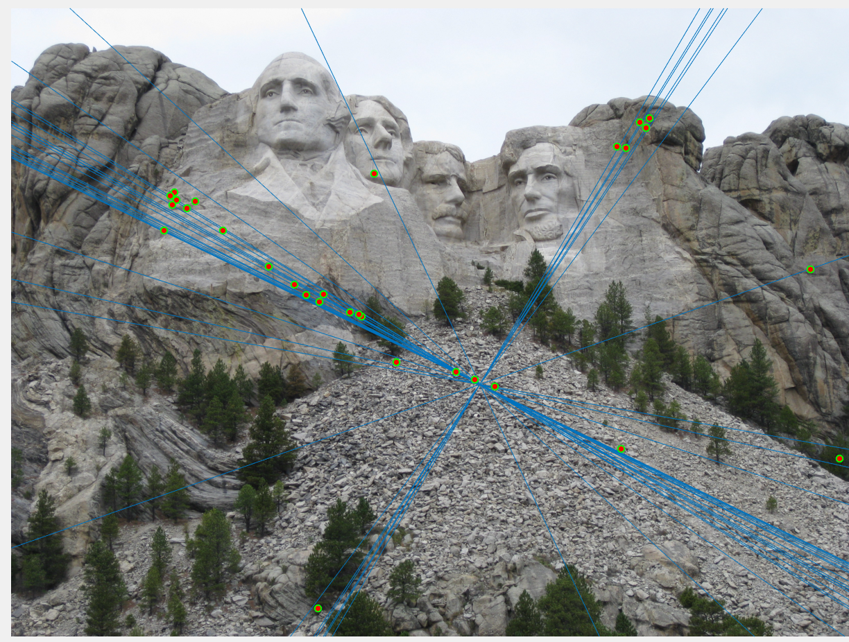
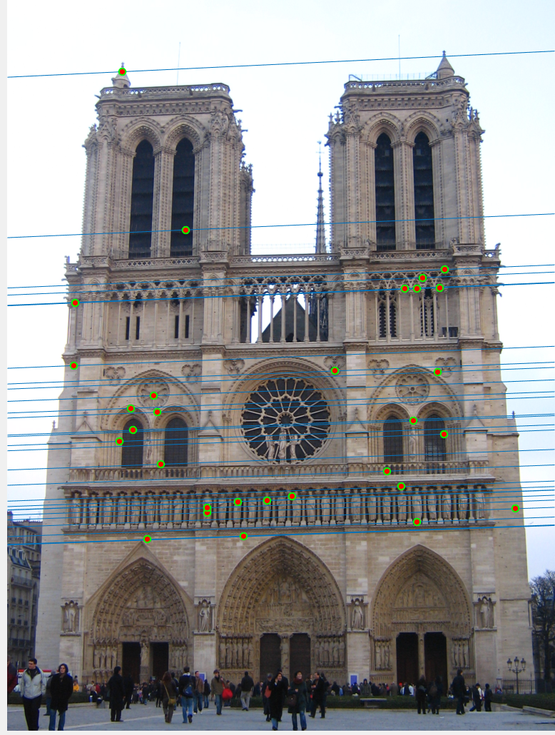
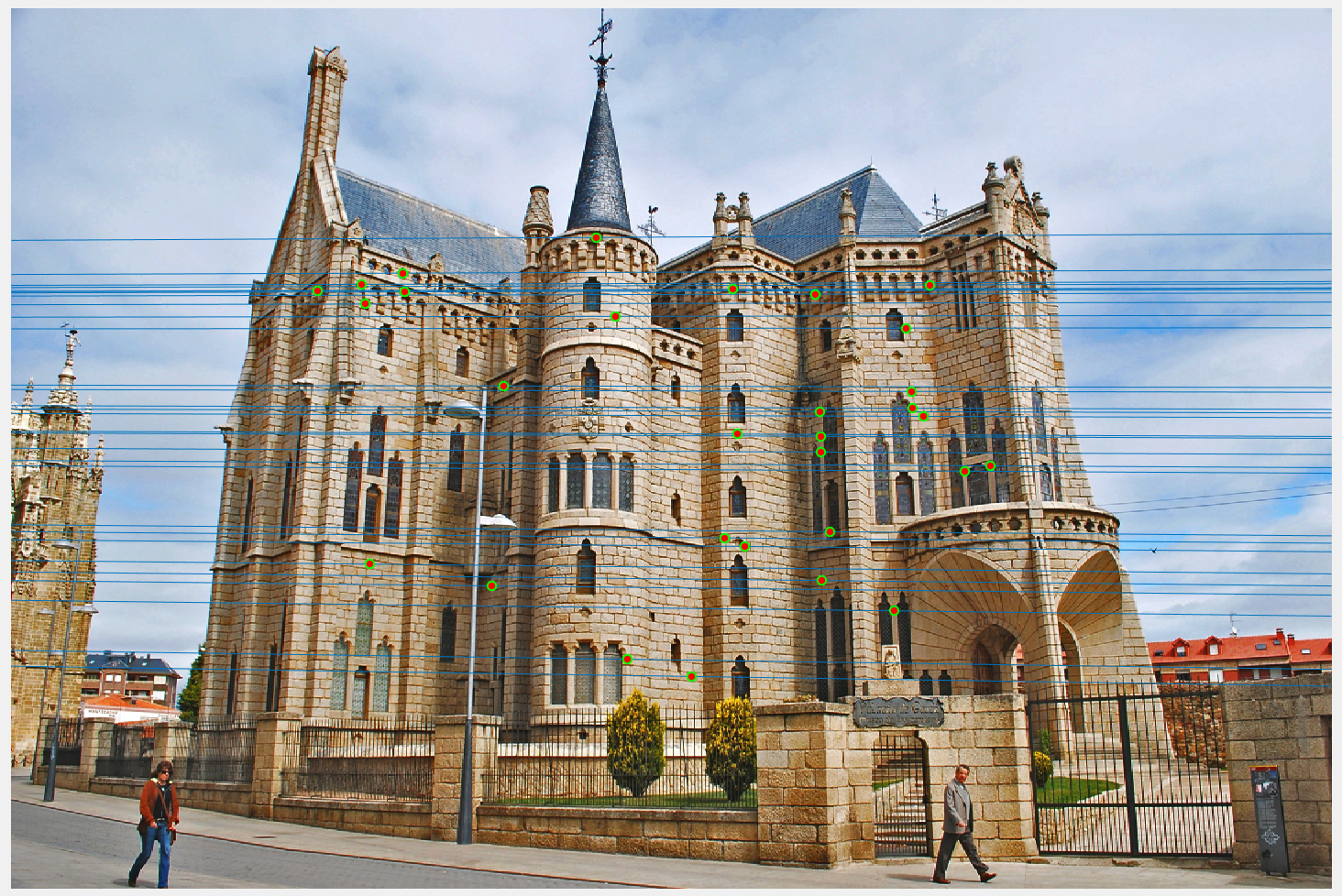
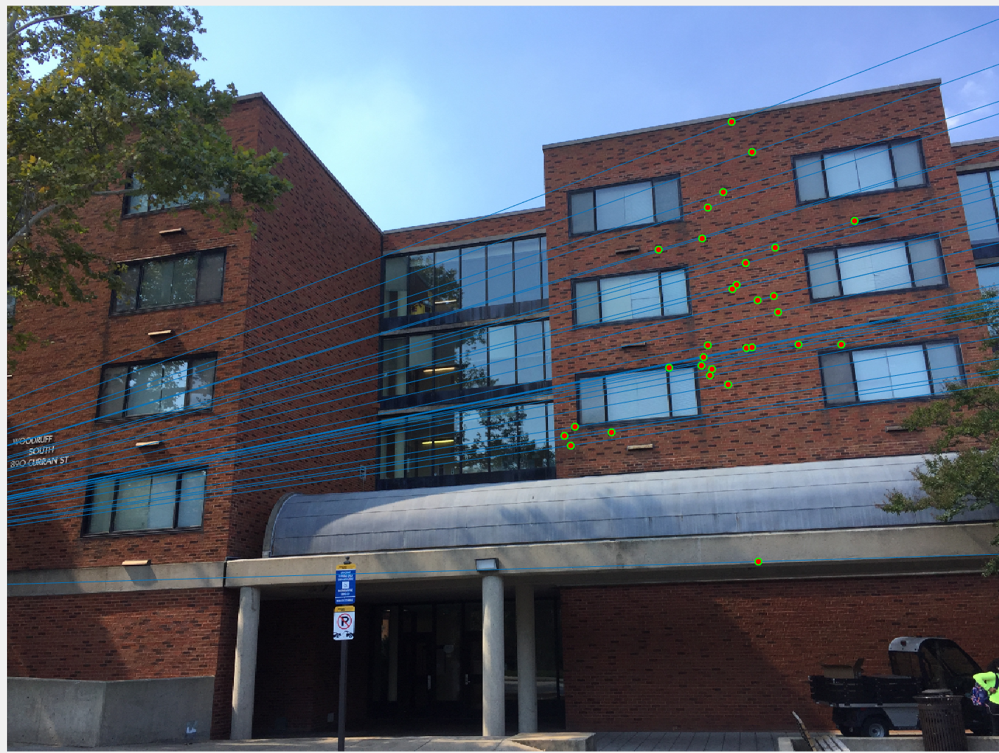
In this method, we first find interest points, and their SIFT features for both the images. This can be done using vlfeat package for MATLAB. Once we obtain the corresponding matches between both the images, we use these points without any processing with 8-point algorithm. Figure 8 shows the SIFT points, and the epipolar lines using the estimated Fundamental Matrix. We see that the lines here do not exactly pass through the corner points.
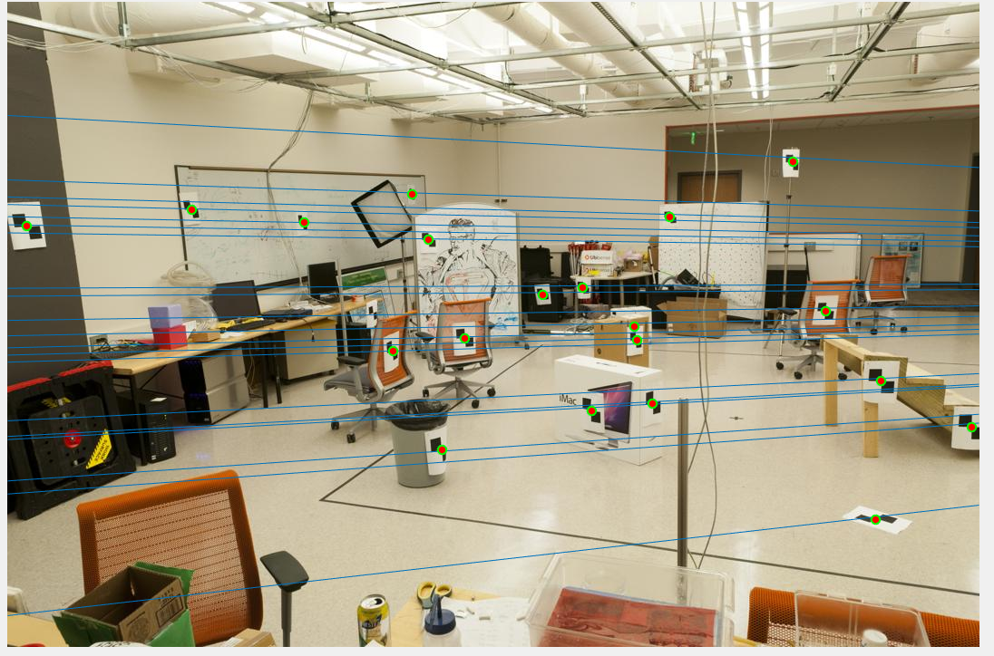
Figure 8(a): Epipolar lines of image 1 without using normalization. |
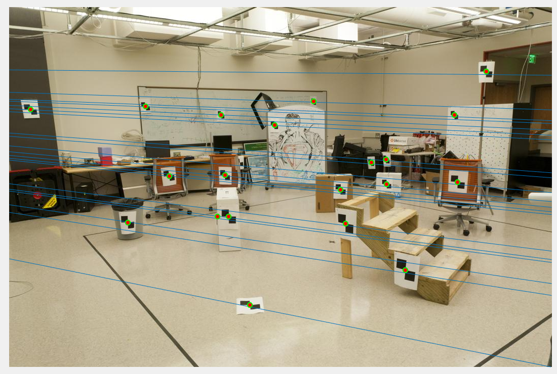
Figure 8(b): Epipolar lines of image 2 without using normalization. |
2. Fundamental Matrix estimation WITH normalization:
Normalization of interest points involves mean centering it, and making the variance of the points equal to 1. The benefit of normalization is that all the points are within unit distance, and do not have any offset. Thus, any processing done on the points now will effect all the points equally. We normalize the points by mean centering them, and scaling them such that the euclidean distance between them is limited to 1. This is done by constructing a transformation matrix using the mean and variance of the points as shown below in Equation 4.

Equation 4: Normalization of coordinates
After Normalization, the 8-point algorithm is performed as usual on these points, giving us the Fundamental matrix. As this F matrix is for the normalized points, we must convert it back for original points by multiplying the transformation matrix constructed above. The results of the using the same image to construct fundamental matrix and draw the resultant epipolar lines is shown below in Figure 9.
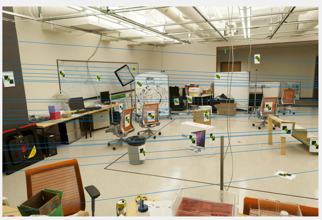
Figure 9(a): Epipolar lines of image 1 using normalization. |
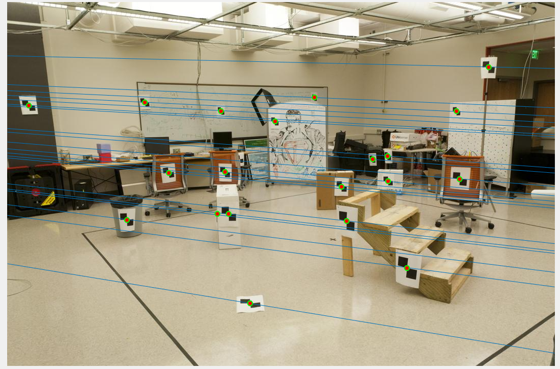
Figure 9(b): Epipolar lines of image 2 using normalization. |
Comparison in performance of normalization and non-normalization:
As we can see in Figures 8 and 9, the interest points are same for both the figures, but we see that the epipolar lines constructed are slightly off centre and do not exactly pass the interest points in the case where we dont use normalization. This can be seen visually by zooming in on specific points of the images in figures 8 and 9 as shown below in figure 10.
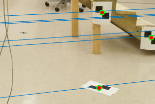
|

|
Figure 10: Zooming in on specific interest points where epipolar lines can be seen to be off.
To Clearly observe the difference between normalized and non-normalized, we add some random noise to both the image and then estimate the fundamental matrix. The results of Noisy interest points without normalization is shown in figure 11, and with normalization is shown in figure 12.
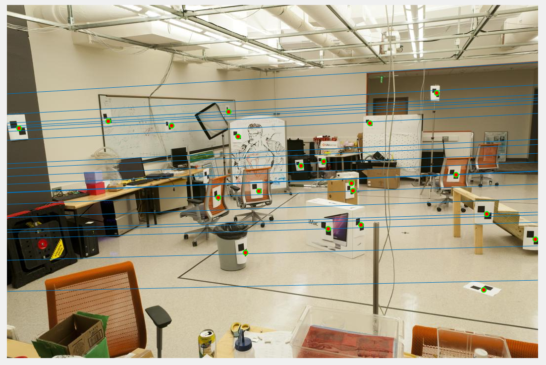
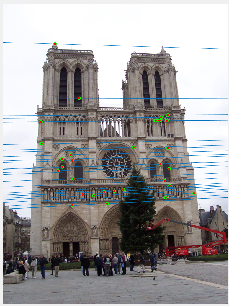
Figure 11(a): Epipolar lines of image 1 with random noise without using normalization. |
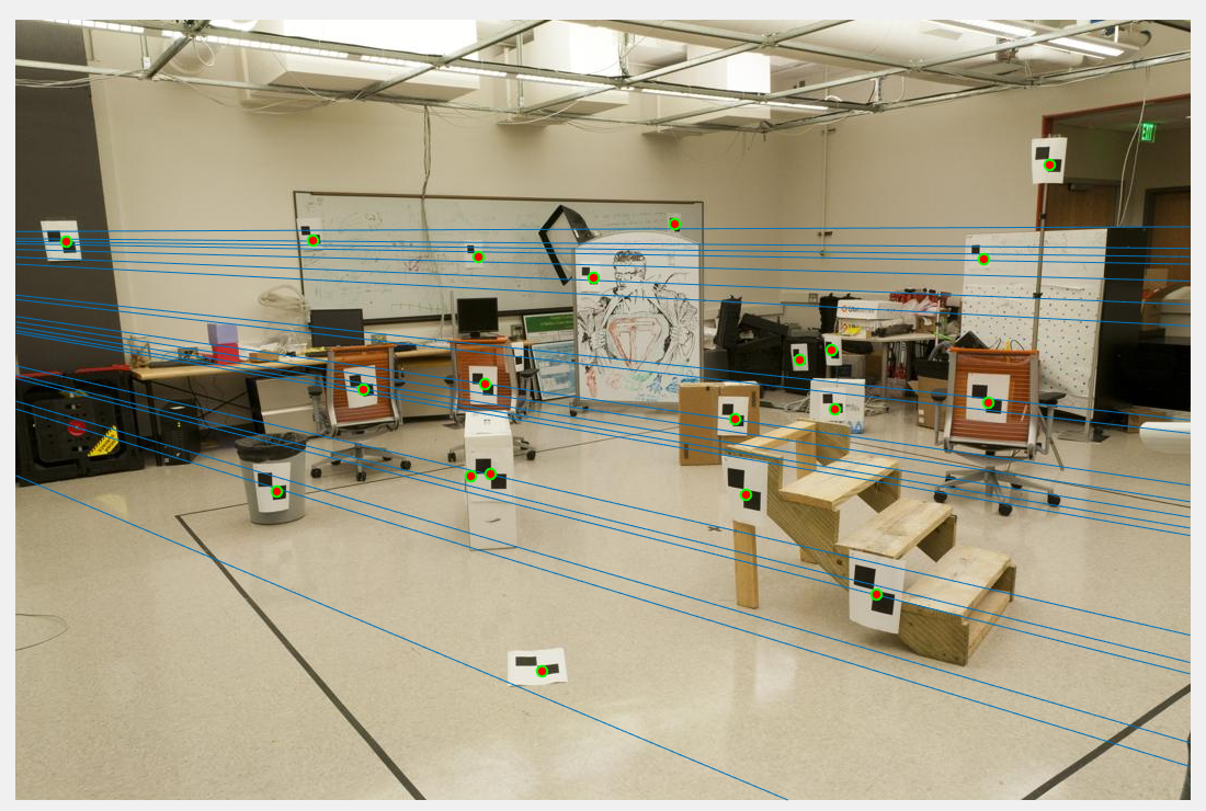
Figure 11(b): Epipolar lines of image 2 with random noise without using normalization. |
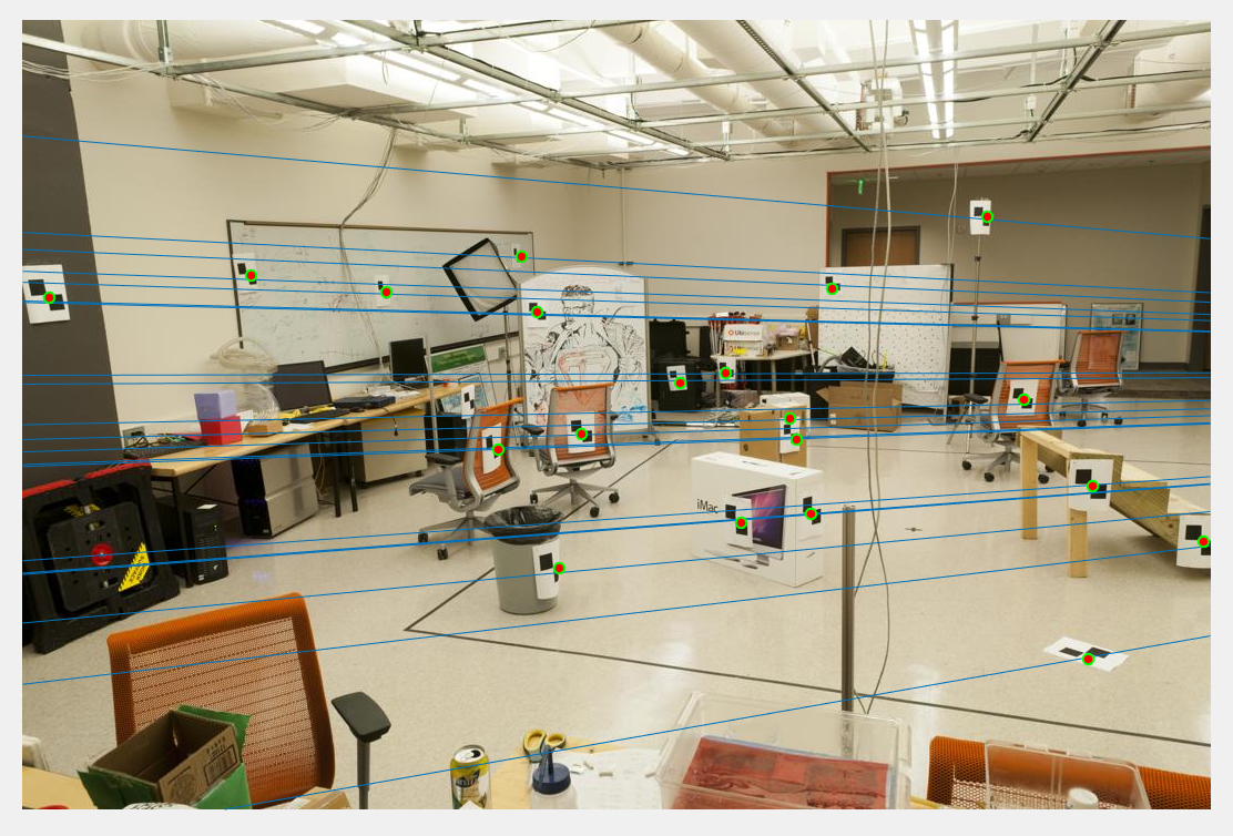
Figure 12(a): Epipolar lines of image 1 with random noise and using normalization. |
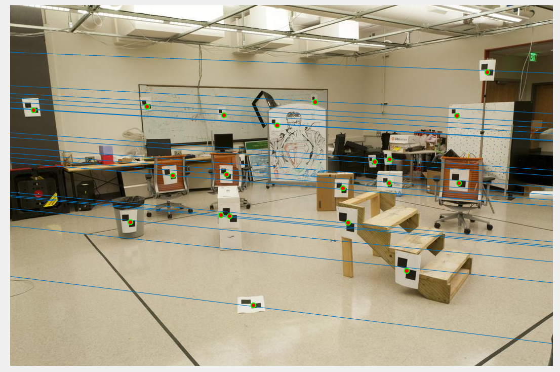
Figure 12(b): Epipolar lines of image 2 with random noise and using normalization. |
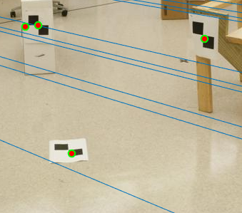
Figure 13(a): Zoomed part of image with Noise and No normalization. |
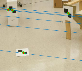
Figure 13(b): Zoomed part of Image with Noise and Normalization. |
Here, we can clearly see that in the case without normalization (figure 11), many lines do not pass the points. Using normalization on the other hand, all the lines pass the points accurately. Zooming in to observe more clearly, we see figure 13 shows the difference between normalization and non-normalization of interest points.
Result in a Table:
1. Without Normalization:
1.a Without Random Noise
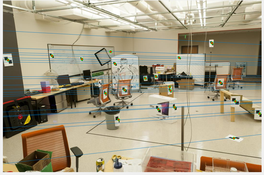
Figure 14(a): Epipolar lines of image 1 without normalization, without noise |
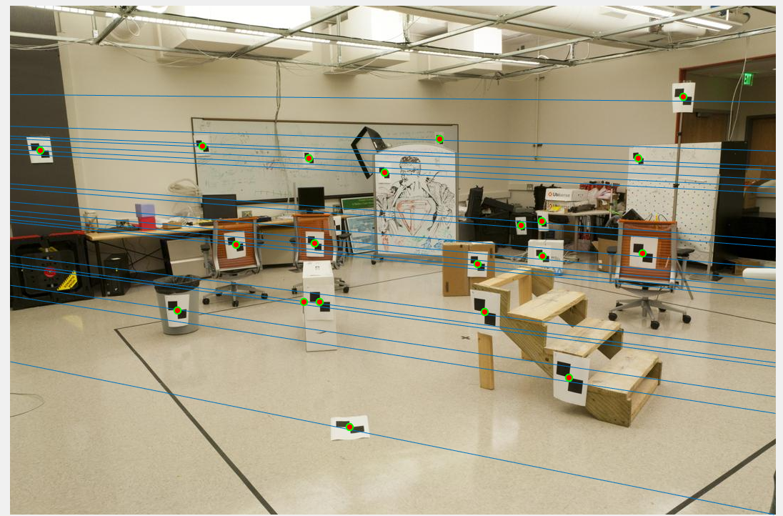
Figure 14(b): Epipolar lines of image 2 without normalization, without noise |
1.b. With Random Noise
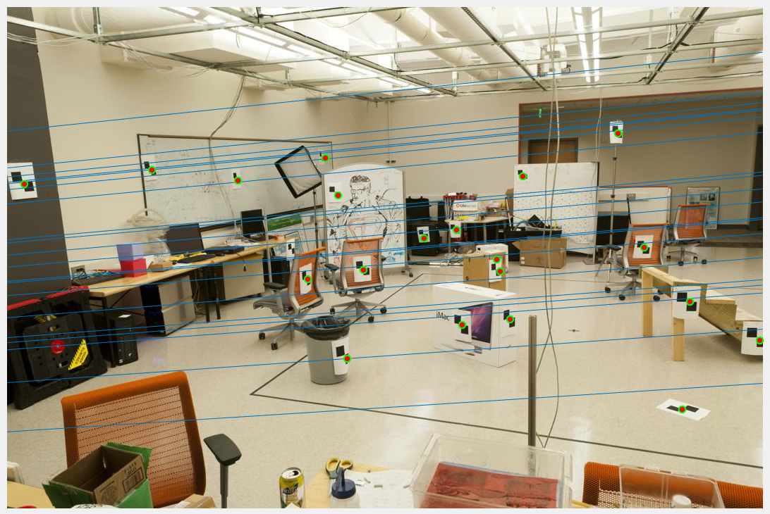
Figure 15(a): Epipolar lines of image 1 without normalization, with noise. |
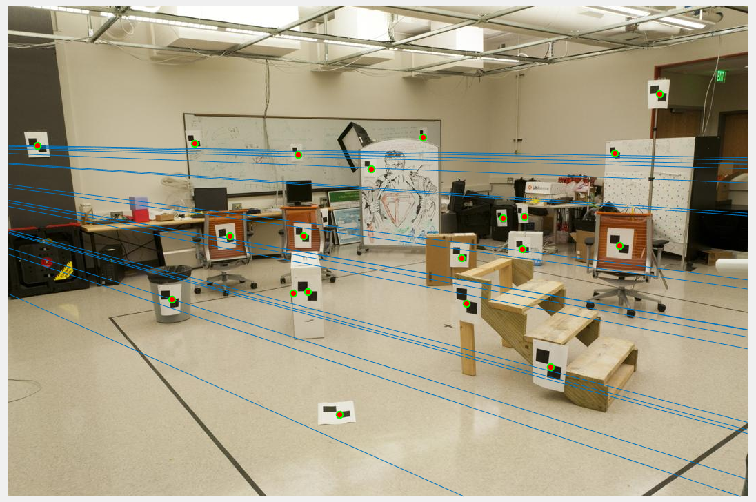
Figure 15(b): Epipolar lines of image 2 without normalization, with noise. |
2. With Normalization
2.a Without Random Noise

Figure 16(a): Epipolar lines of image 1 with normalization, without noise. |
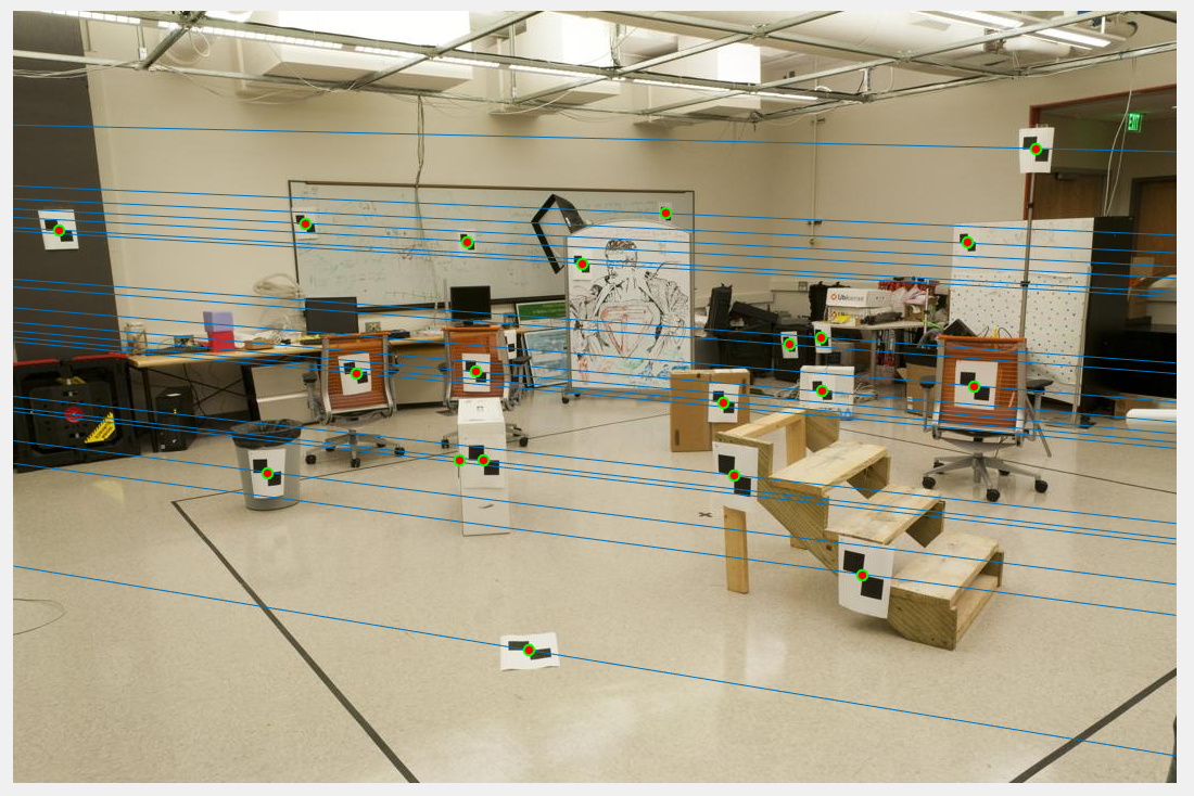
Figure 16(b): Epipolar lines of image 2 with normalization, without noise. |
2.b With Random Noise
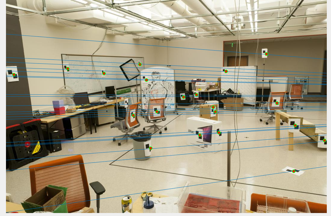
Figure 17(a): Epipolar lines of image 1 with normalization, with noise. |

Figure 17(b): Epipolar lines of image 2 with normalization, with noise. |
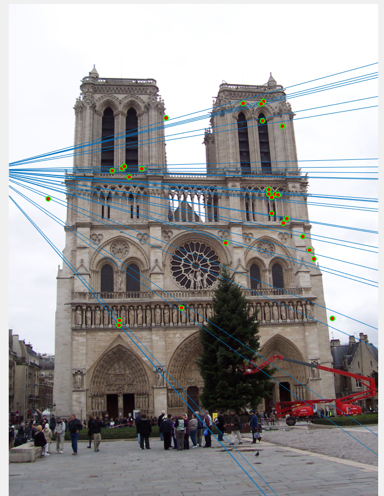
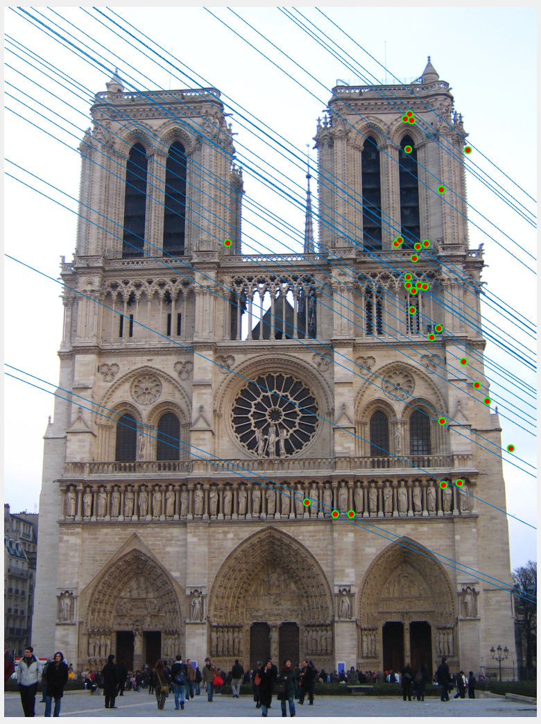
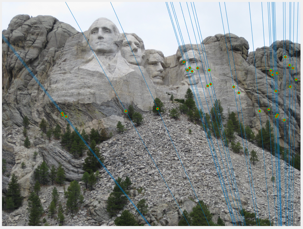
III. Using RANSAC to find Best Estimate of Fundamental Matrix.
For estimating Fundamental Matrix, we must have at least 8 sets of matching points between both the images. The matrix F has 9 independent values in it, but since we're dealing with homogeneous coordinate system, we're only interested upto a certain scale. Which means that there are effectively 8 independent values in F.Thus we need only 8 points to estimate fundamental matrix. SIFT will give us many more than 8 matches. Thus we use RANSAC to randomly pick 8 points, and construct the fundamental matrix using them. A good Fundamental matrix is one which will adhere to equation 5. Although we wont get exactly 0, we can have a soft bound by thresholding the values obtained, and computing the number of inliers. This is done using equation 6. Using multiple iterations, the best F matrix is one that gives us maximum number of inliers. Threshold value is a fre parameter here, and is tuned by checking the result.
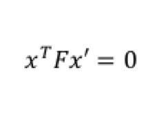
Equation 5: Equation for Fundamental Matrix.
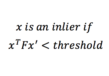
Equation 6: Equation for distance metric.
Once we have out best fundamental matrix, we pick 30 matches with lowest values of the distance metric.
Result in a Table:
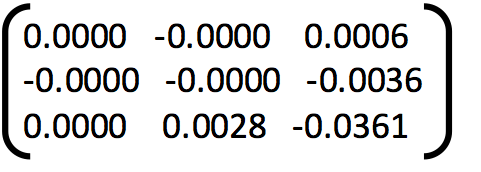
1. Example of poor fundamental matrix:
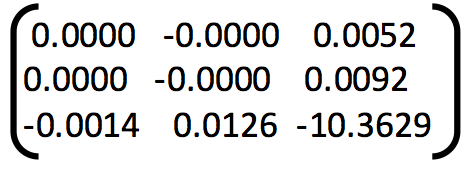
Fundamental Matrix =
Number of inliers = 36
Number of iterations of RANSAC = 1
Threshold = 0.05
|
2. Example of poor fundamental matrix:
Fundamental Matrix =
Number of inliers = 29
Number of iterations of RANSAC = 5
Threshold = 0.05
|
3. Example of poor fundamental matrix:
Fundamental Matrix =
Number of inliers = 73
Number of iterations of RANSAC = 20
Threshold = 0.05
|
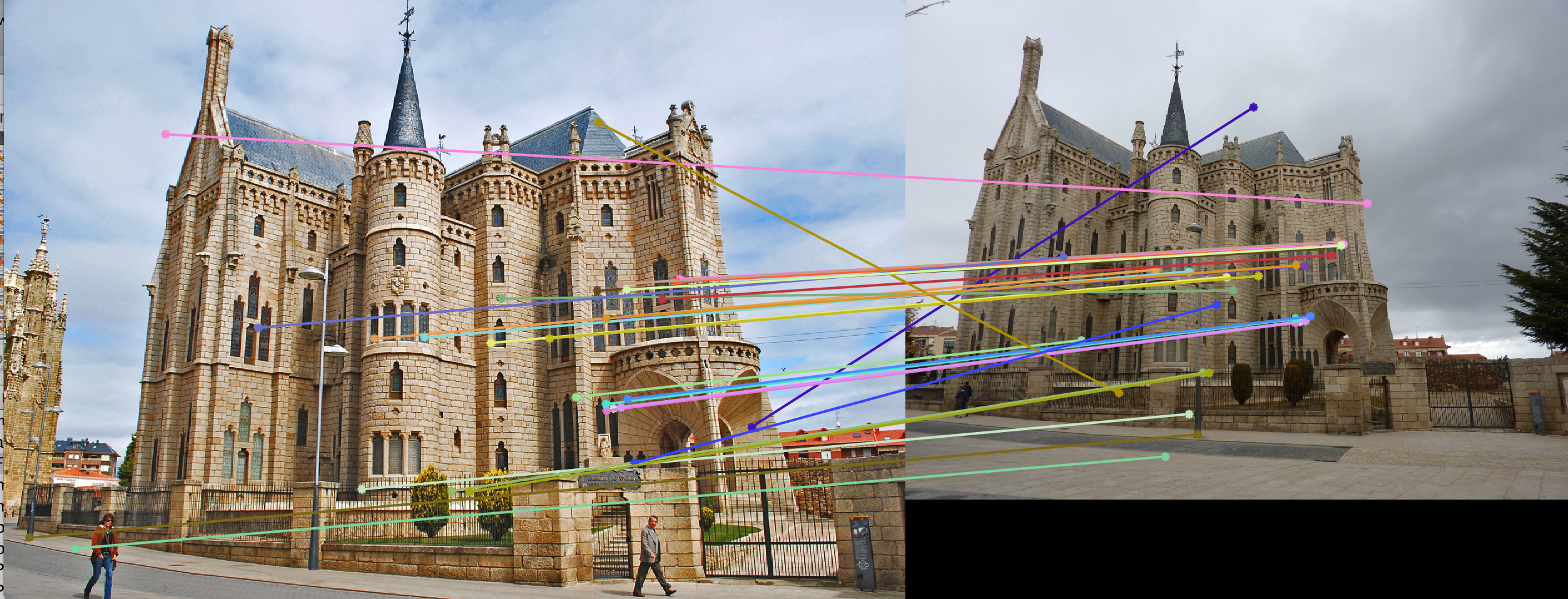
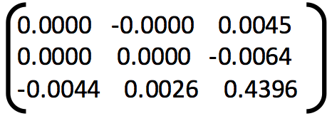
4. Example of good fundamental matrix:
Fundamental Matrix =

Number of inliers = 672
Number of iterations of RANSAC = 1000
Threshold = 0.05
|
5. Example of good fundamental matrix:
Fundamental Matrix =
Number of inliers = 689
Number of iterations of RANSAC = 1000
Threshold = 0.05
|
6. Example of good fundamental matrix:
Fundamental Matrix =
Number of inliers = 522
Number of iterations of RANSAC = 1000
Threshold = 0.05
|
6. Example of good fundamental matrix:
Fundamental Matrix =
Number of inliers = 322
Number of iterations of RANSAC = 1000
Threshold = 0.05
|
We can see from the above results that with greater number of RANSAC iterations, we get Fundamental Matrices with more number of inliers. Thus RANSAC with normalzation gives us good results where the epipolar lines pass the interest points.