Your Name

    
    % Set up regression equations
    n=size(Points_2D,1);

    Xl = zeros(2*n,4);
    Xl(1:2:2*n,1:3) = Points_3D;
    Xl(1:2:2*n,4) = 1;

    Xr = zeros(2*n, 4);
    Xr(2:2:2*n,4 )= 1;
    Xr(2:2:2*n,1:3) = Points_3D;

    uvX = zeros(2*n,3);
    uvX(1:2:2*n,:) = Points_3D;
    uvX(2:2:2*n,2:3) = Points_3D(:,2:3);
    uvX(2:2:2*n,1) = Points_3D(:,3);

    Points_2DT = Points_2D';
    X = [Xl Xr (-bsxfun(@times,uvX,Points_2DT(:)))];

    % Solve regression equations
    M_col = X\Points_2DT(:);
    % This part is to ensure that the values we've found are set in their right places in the projection matrix
    M = ones(4,3);
    M(1:11) = M_col;
    M = M';
    
    

    Q = M(:,1:3);
    m4 = M(:,4);
    Center = -(Q^-1) * m4;
    

Estimating the fundamental matrix

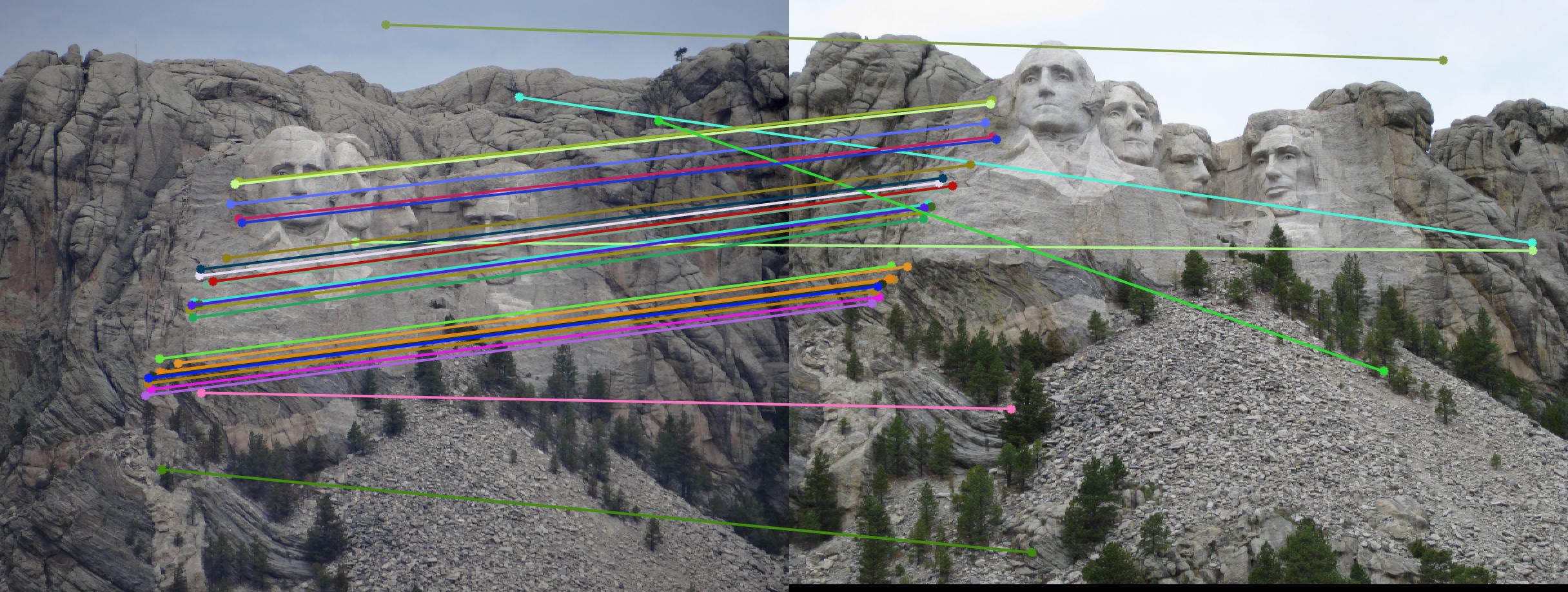
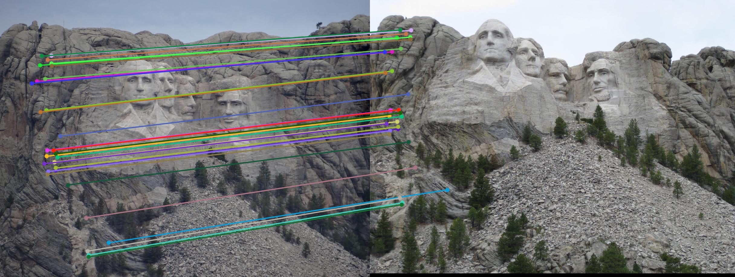
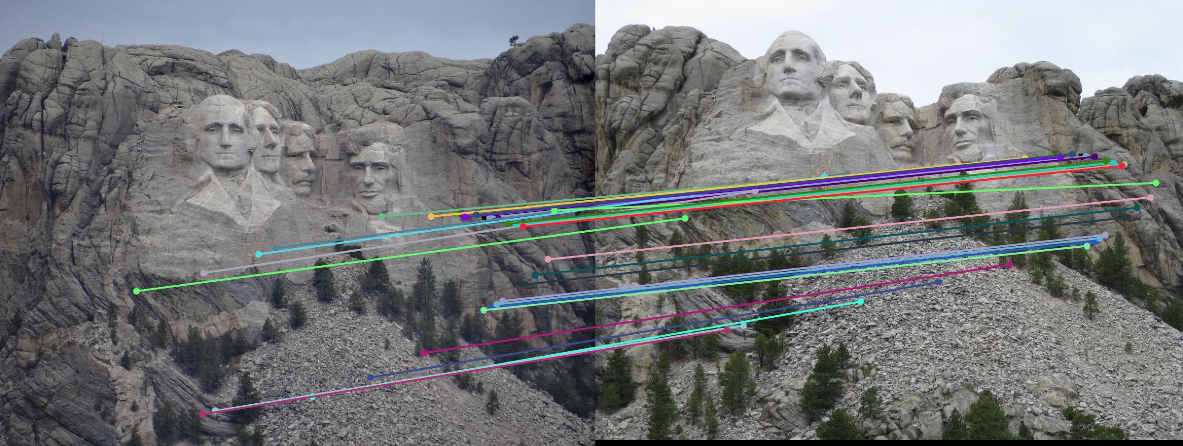
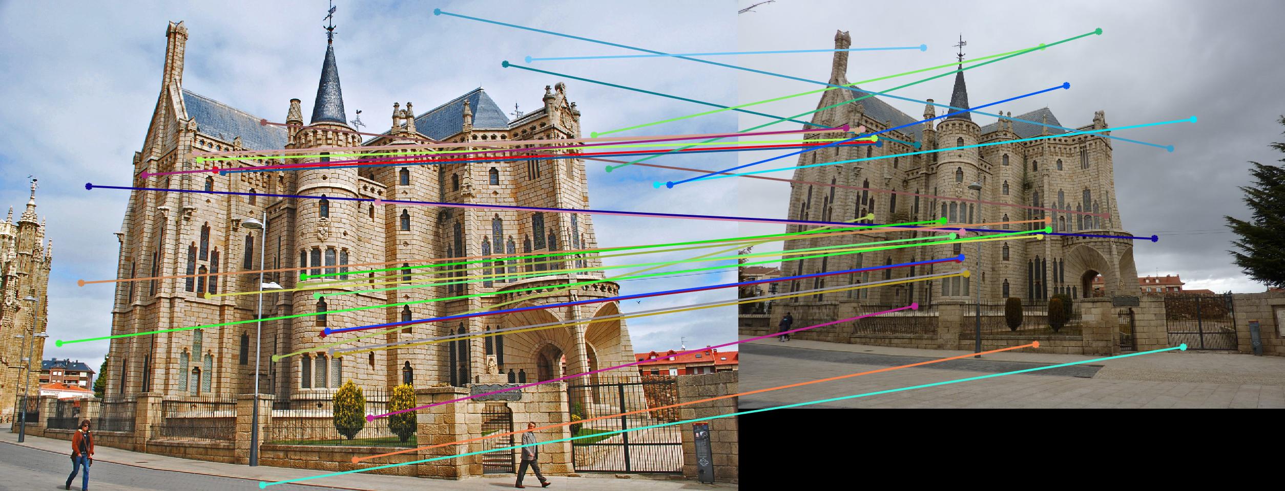
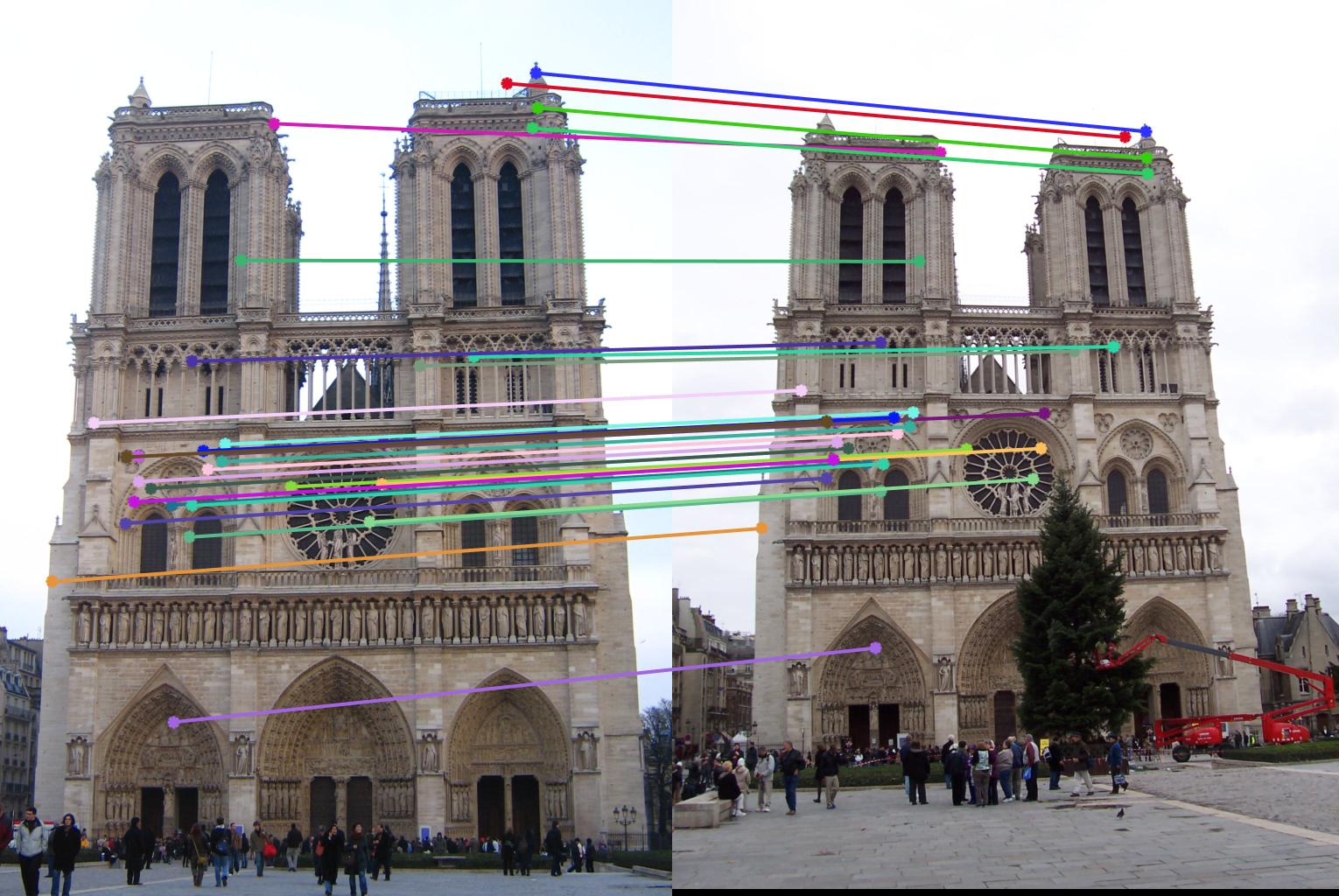
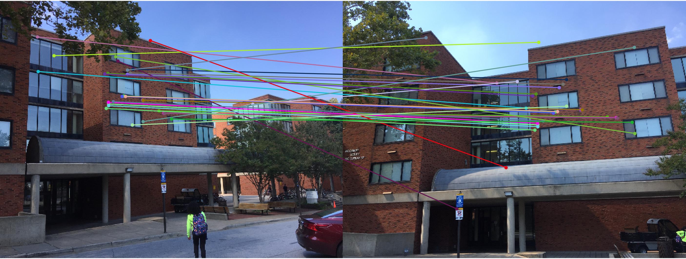
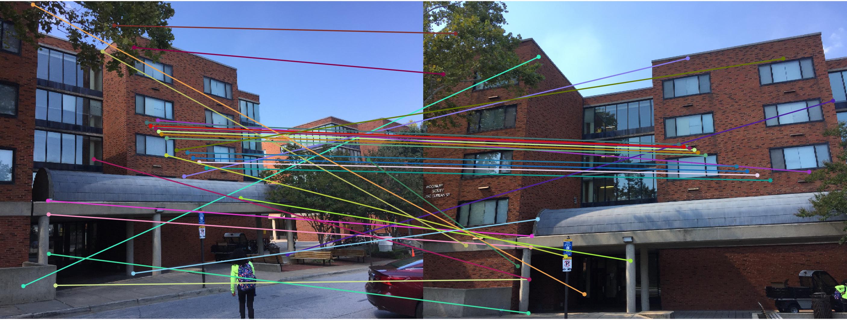
Given a set of matching points in a pair of stereo images, the fundamental matrix gives us the mapping between the two points. That is if [u1, v1] and [u2, v2] are the matching points in two stereo images, the fundamental matrix satisfies the property [u1 v1 1] * F * [u2 v2 1]' = 0.

In this project, we solve for it using the 8 points algorithm. The matrix F has 9 independent values in it, but since we're dealing with homogeneous coordinate system, we're only interested upto a certain scale. Which means that there are effectively 8 independent values in F. Thus 8 correspondence pairs are sufficient to find F. In fact, because F has rank 2, 7 points are sufficient, and the corresponding algorithm is called the seven point algorithm.

The 8 points algorithm is very similar to the algorithm we used to find the projection matrix. Given 8 correspondence pairs, we set up the regression equations and solve for F. The only additional step is that we need to constrain F to be of rank 2.

The matlab code is as follows:

        % Set up regression equation
        pa = [Points_a ones(size(Points_a,1),1)];
        pb = [Points_b ones(size(Points_b,1),1)];
        xy = repelem(pa(:,1:2),1,3);
        A = [xy .* repmat(pb,1,2) pb];

        % Solve for F
        [~, ~, V] = svd(A);
        f = V(:, size(V,2));
        F = reshape(f, 3, 3)';

        % Constrain F to have rank 2
        [U, D, V] = svd(F);
        F_matrix = U * diag([D(1,1) D(2,2) 0]) * V';
        

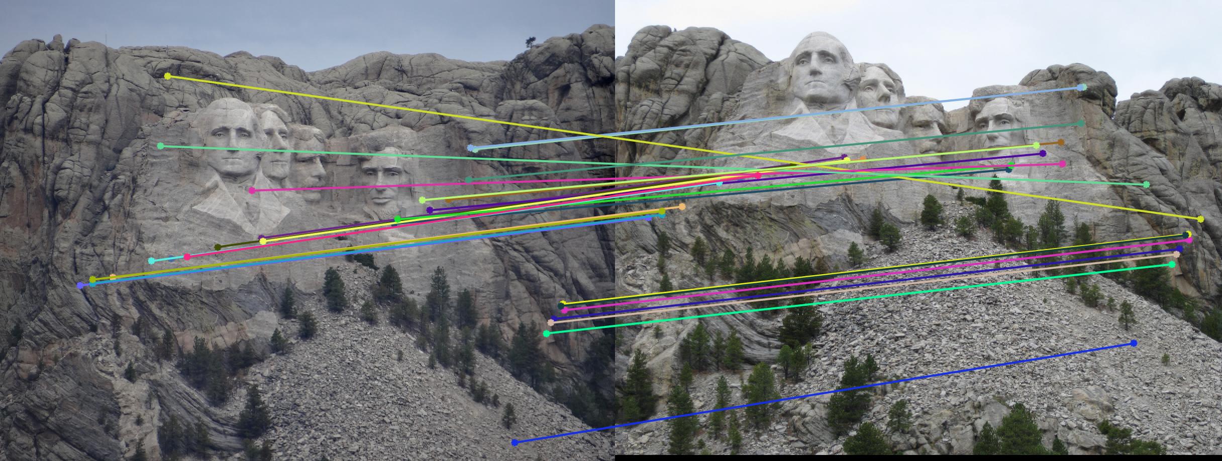
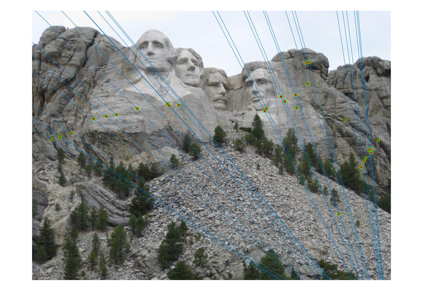
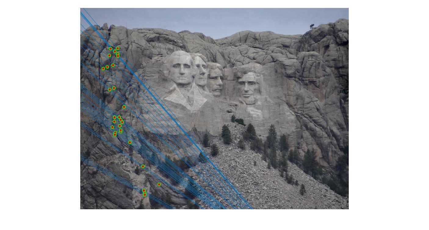
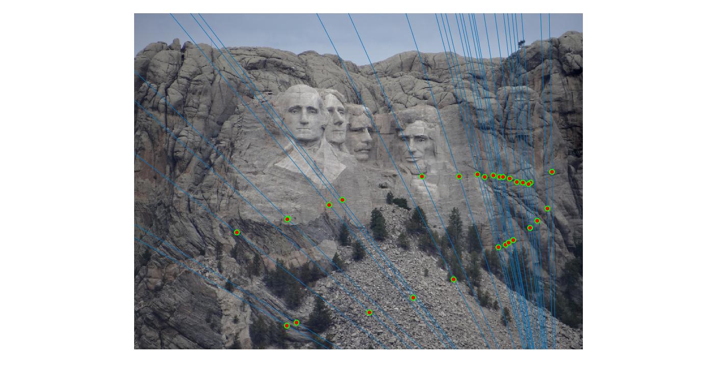
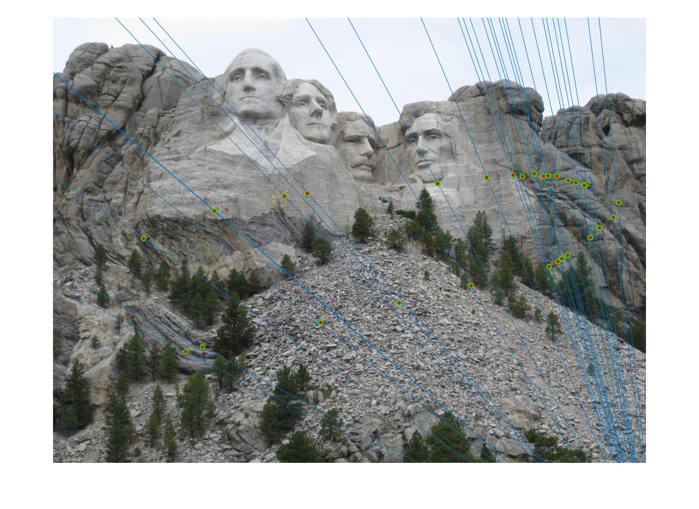
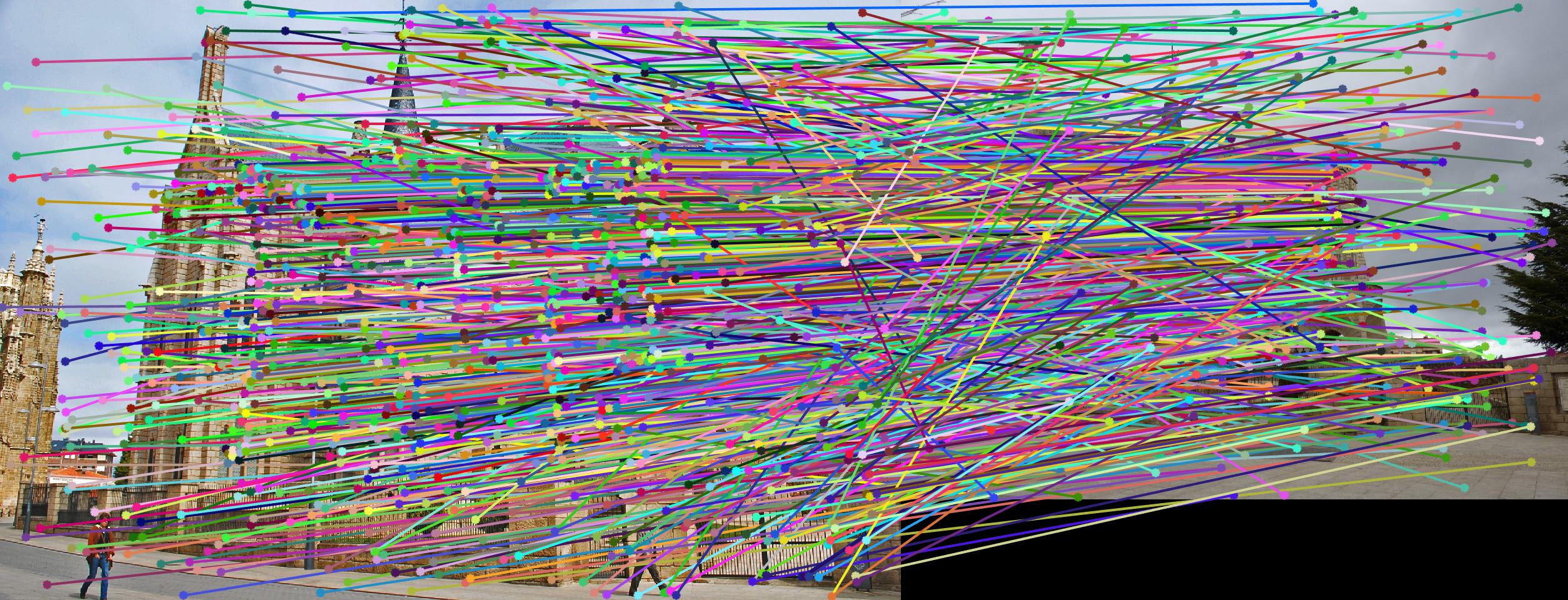
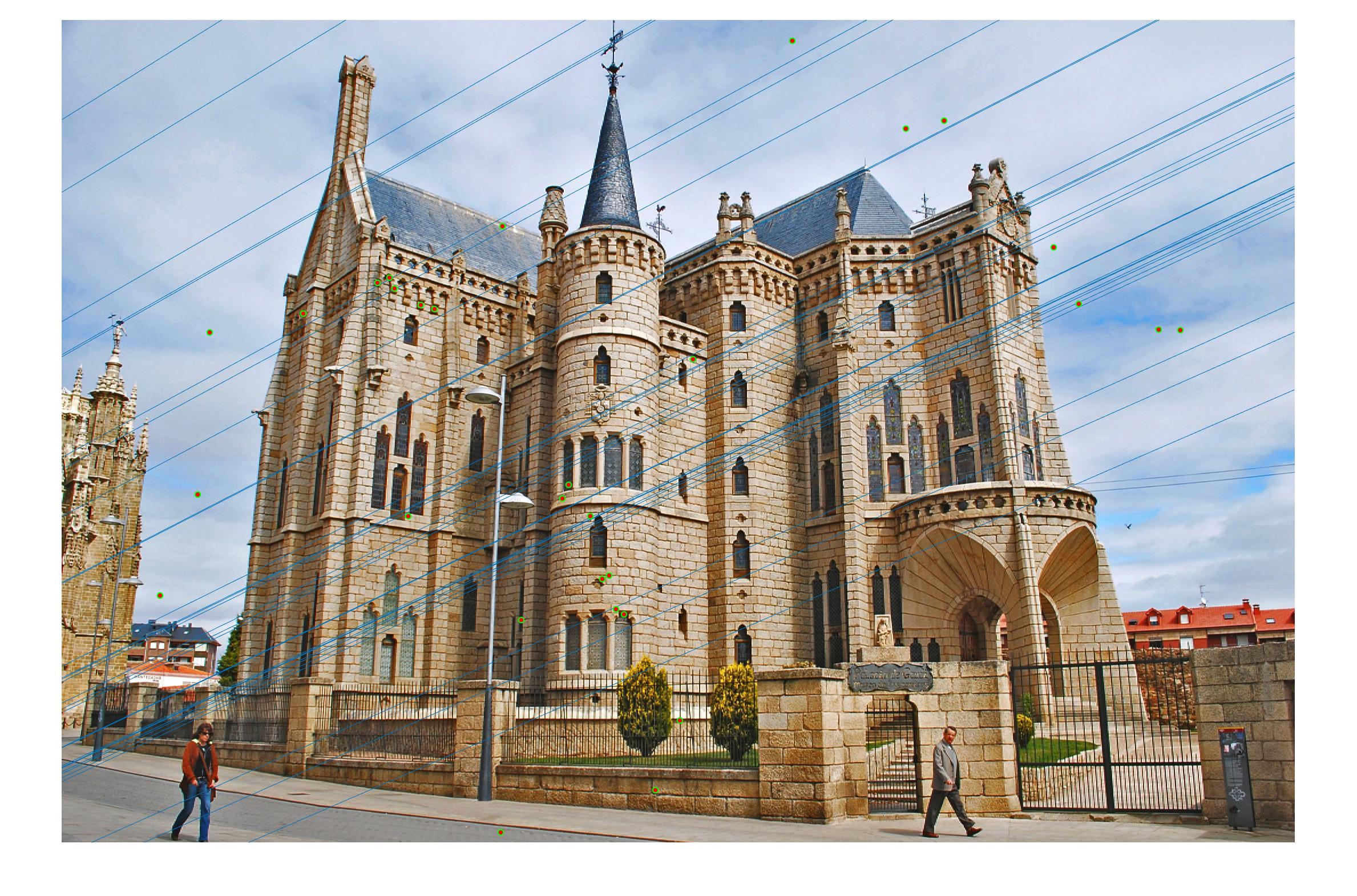
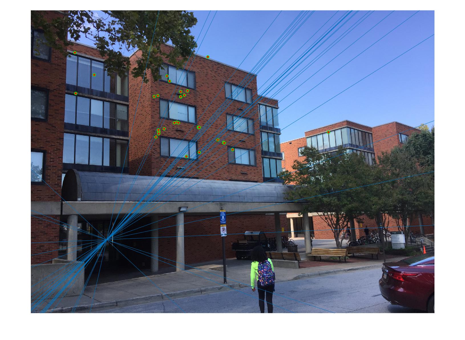
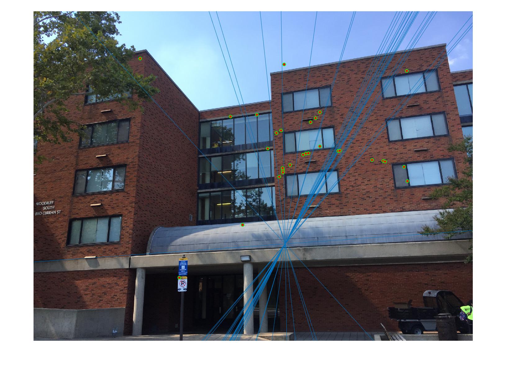
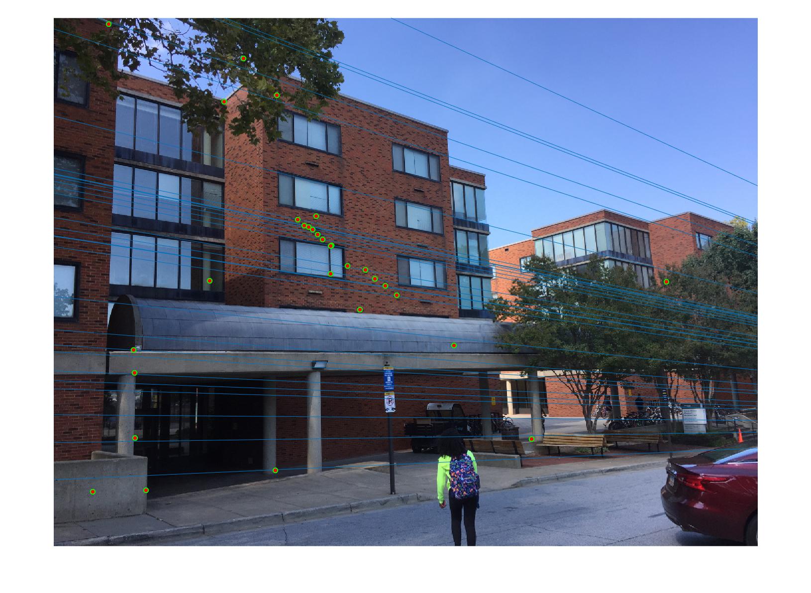
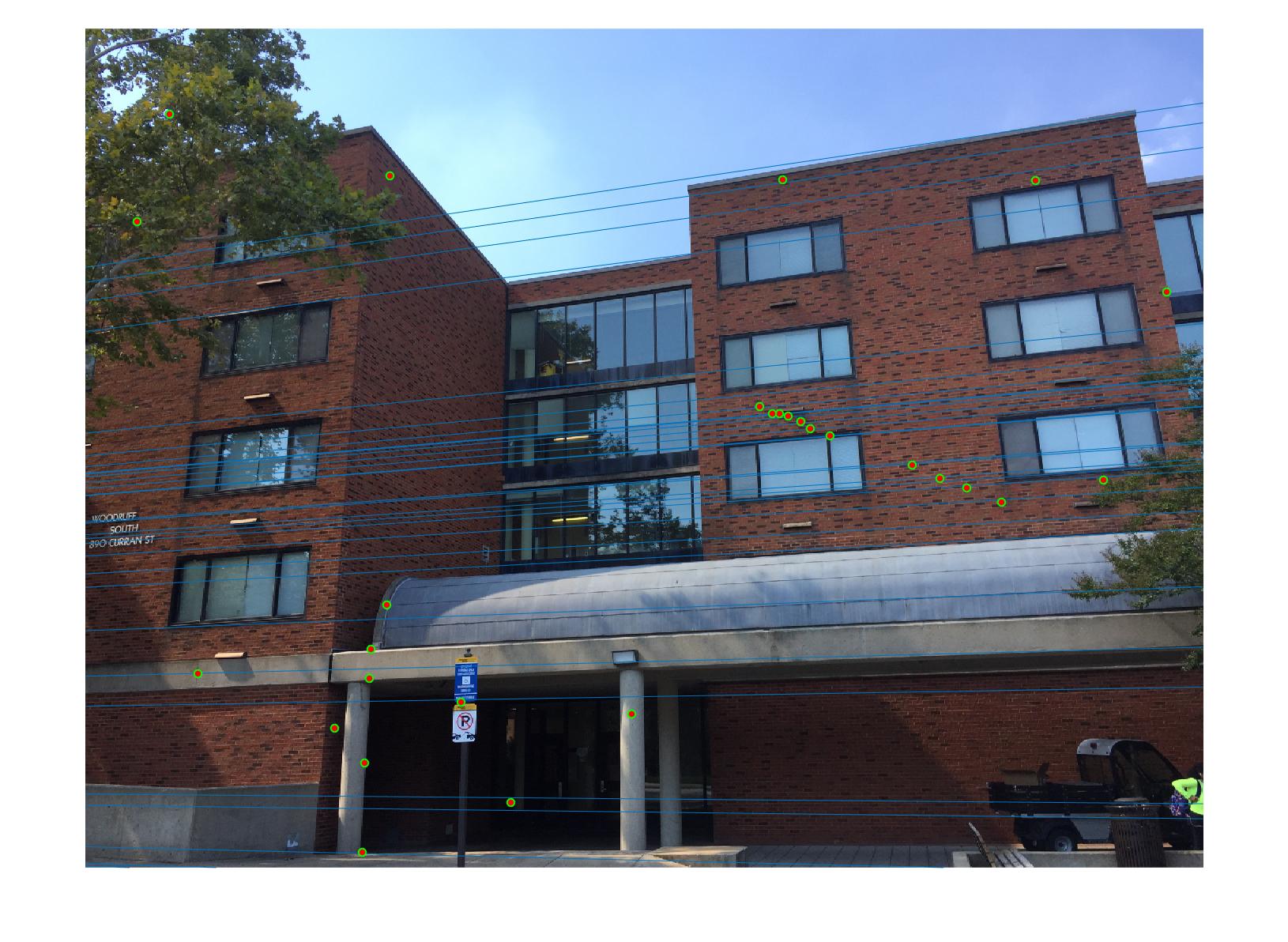
Improving matched features using RANSAC

Feature matching algorithms like SIFT give us a lot of matches. But there are many outliers in these matches. There are various techniques to detect outliers. One of these techniques is RANSAC.

The rnsc algorithm or the RANdom SAmple Consensus algorithm is very simple. For any model fitting problem, in each iteration,

1. randomly sample the minimum number of points required to fit the model. For rnsc this is 8
2. fit the model (find F) using these points
3. setting a threshold, find the ratio of inliers to outliers for the fitted model

Repeat the above procedure until convergence is reached.

The matlab code for this is as follows:

        for i = 1:N
            rand_ind = randsample(size(matches_a,1),s);
            points_a = matches_a(rand_ind, :);
            points_b = matches_b(rand_ind, :);
            F_est = estimate_fundamental_matrix(points_a, points_b, normalize);
            mult = sum([matches_b ones(size(matches_b,1),1)] .* ...
                (F_est * [matches_a ones(size(matches_a,1),1)]')',2);
            mult = abs(mult);
            n_inliers(i) = numel(mult(mult < thresh));
            F_matrices(:,:,i) = F_est;
        end
        

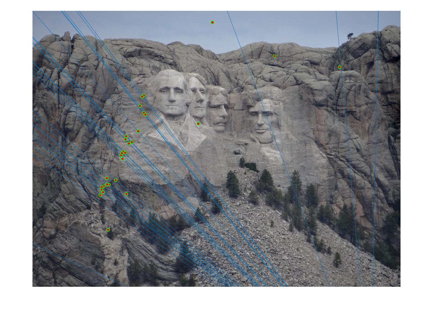
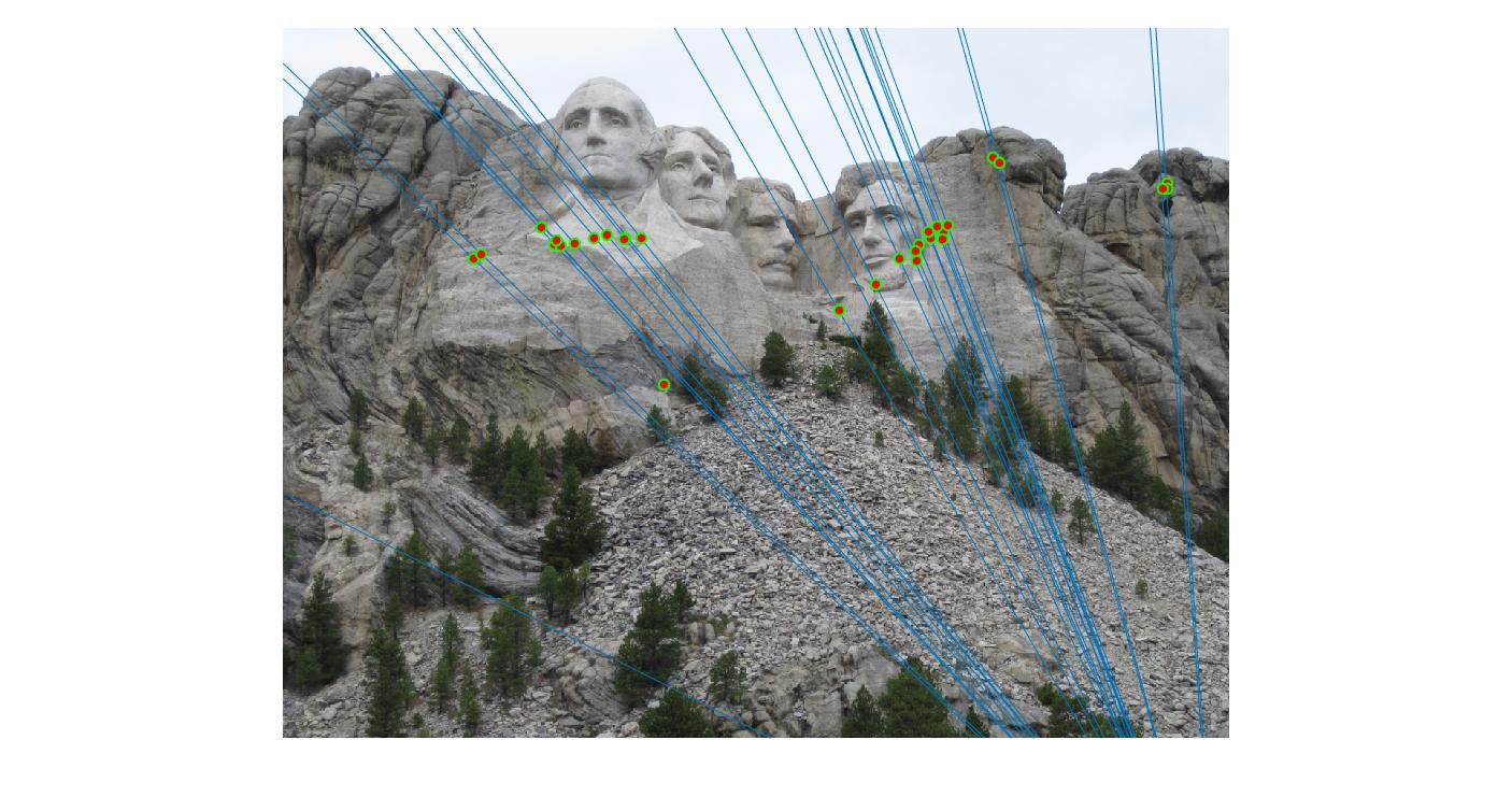
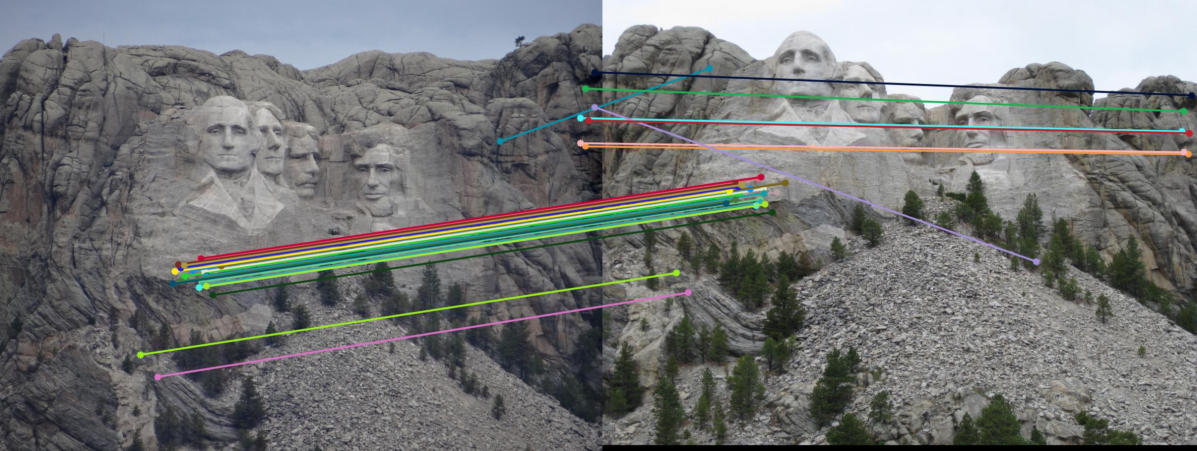
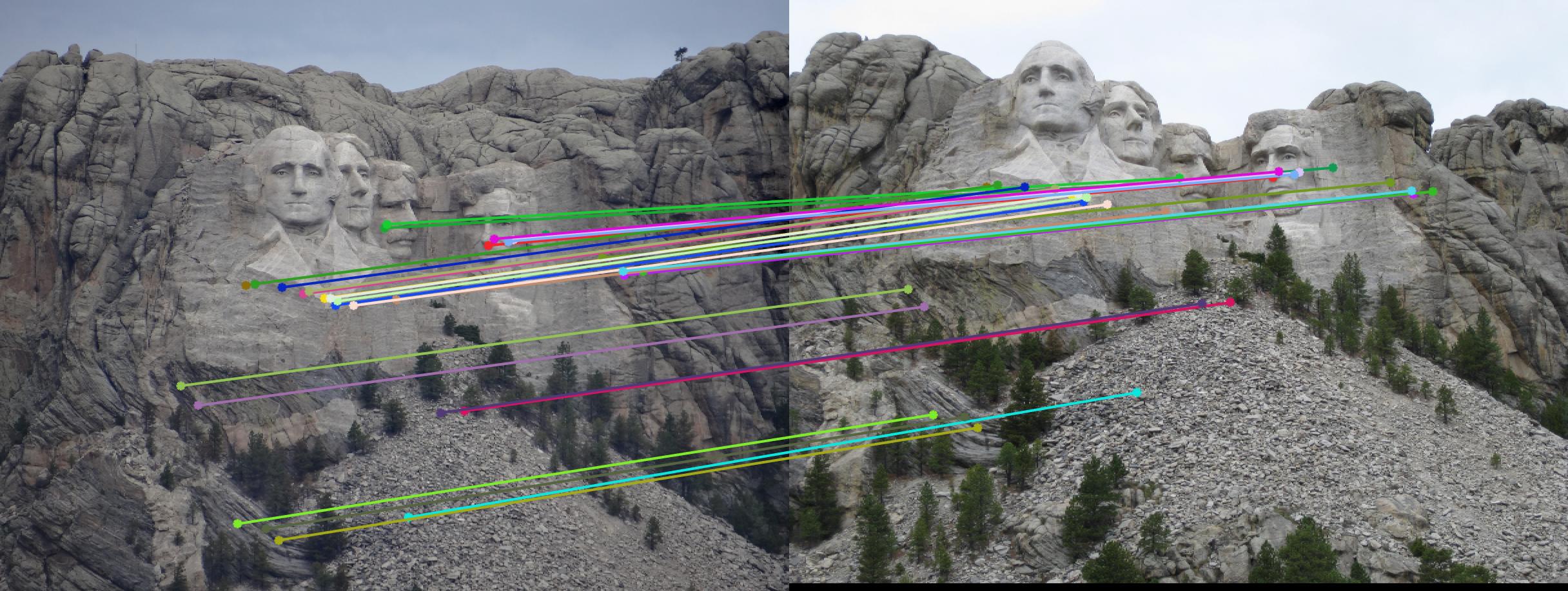
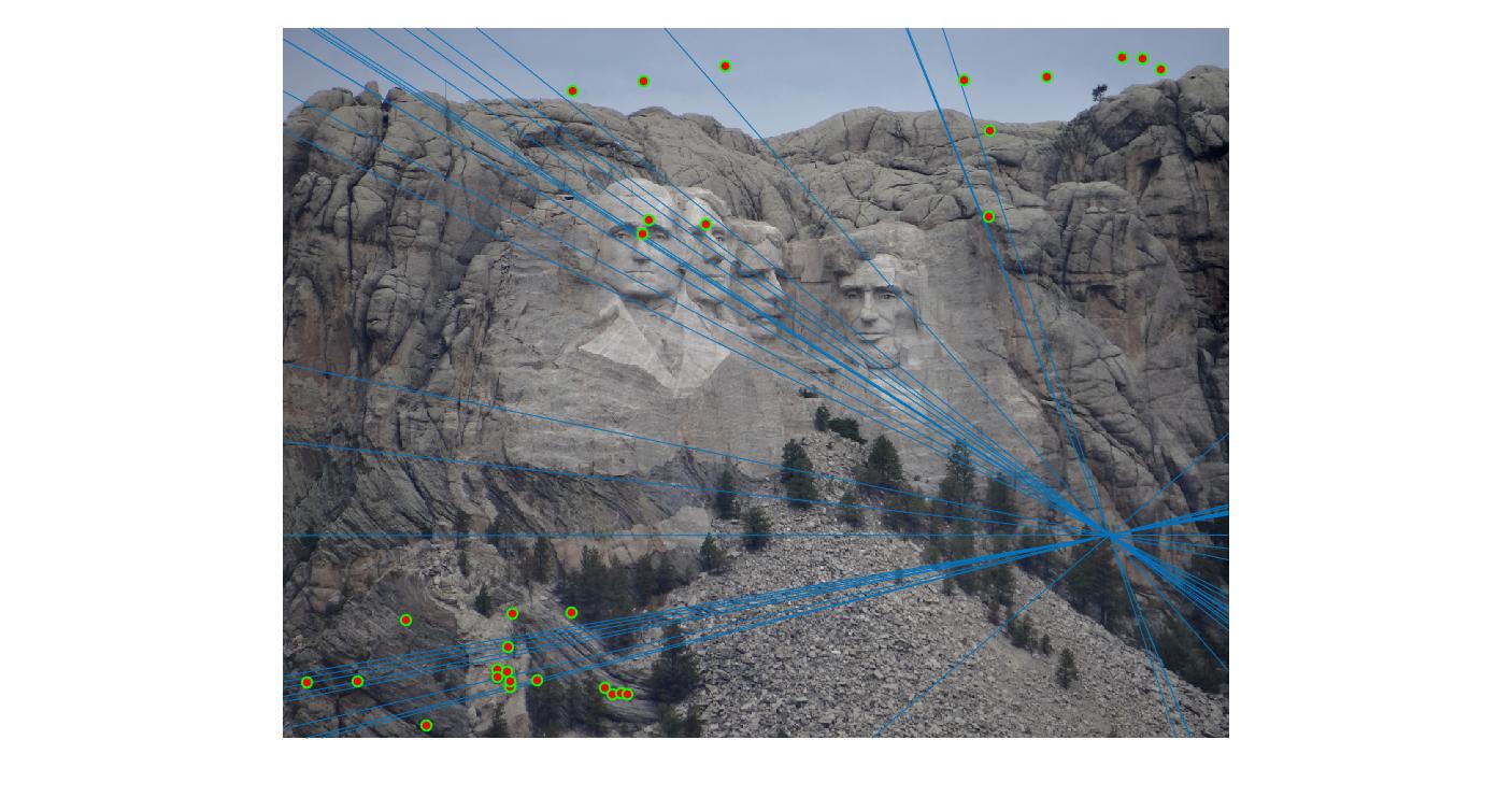
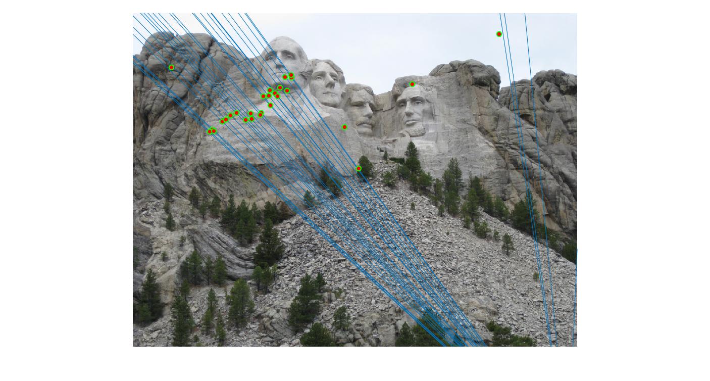
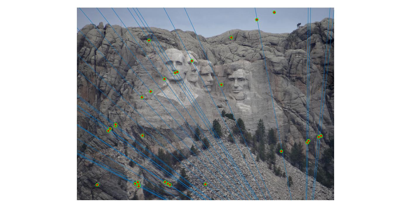
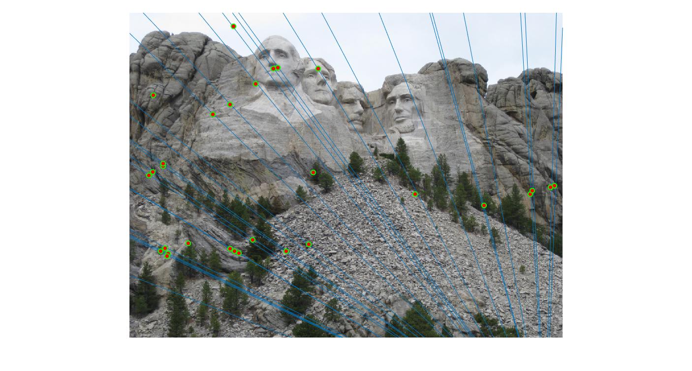
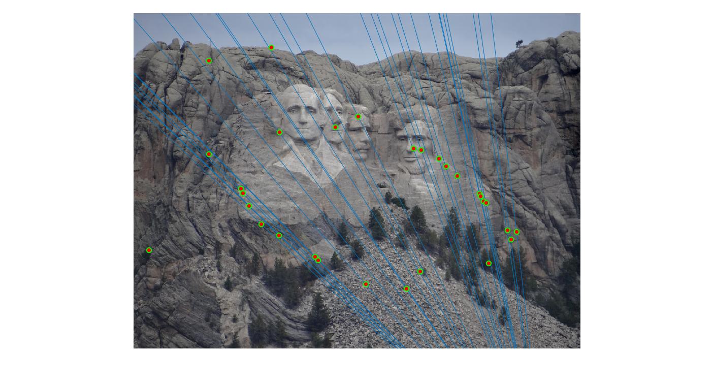
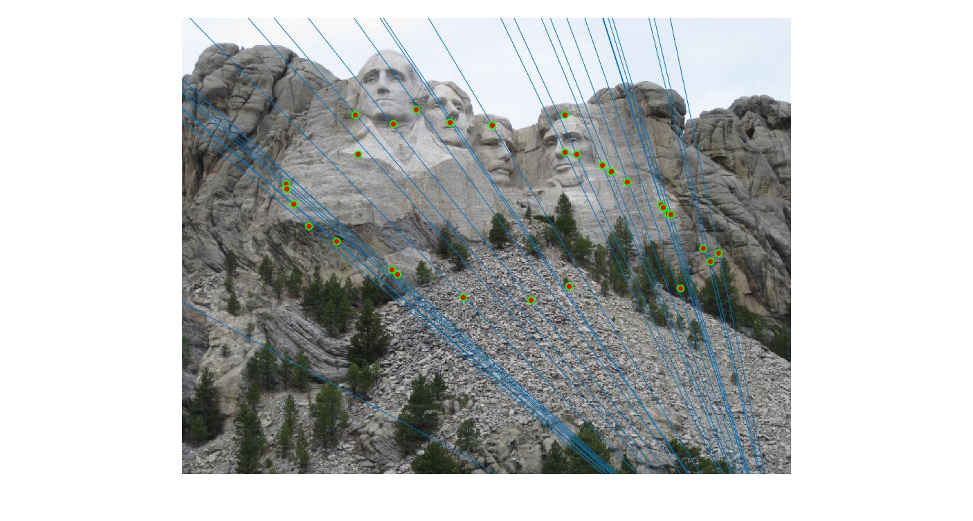
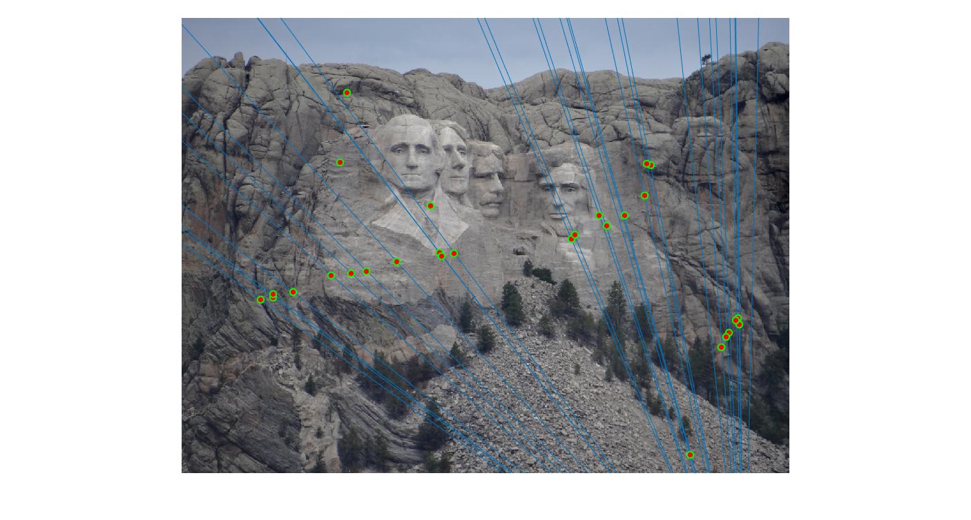
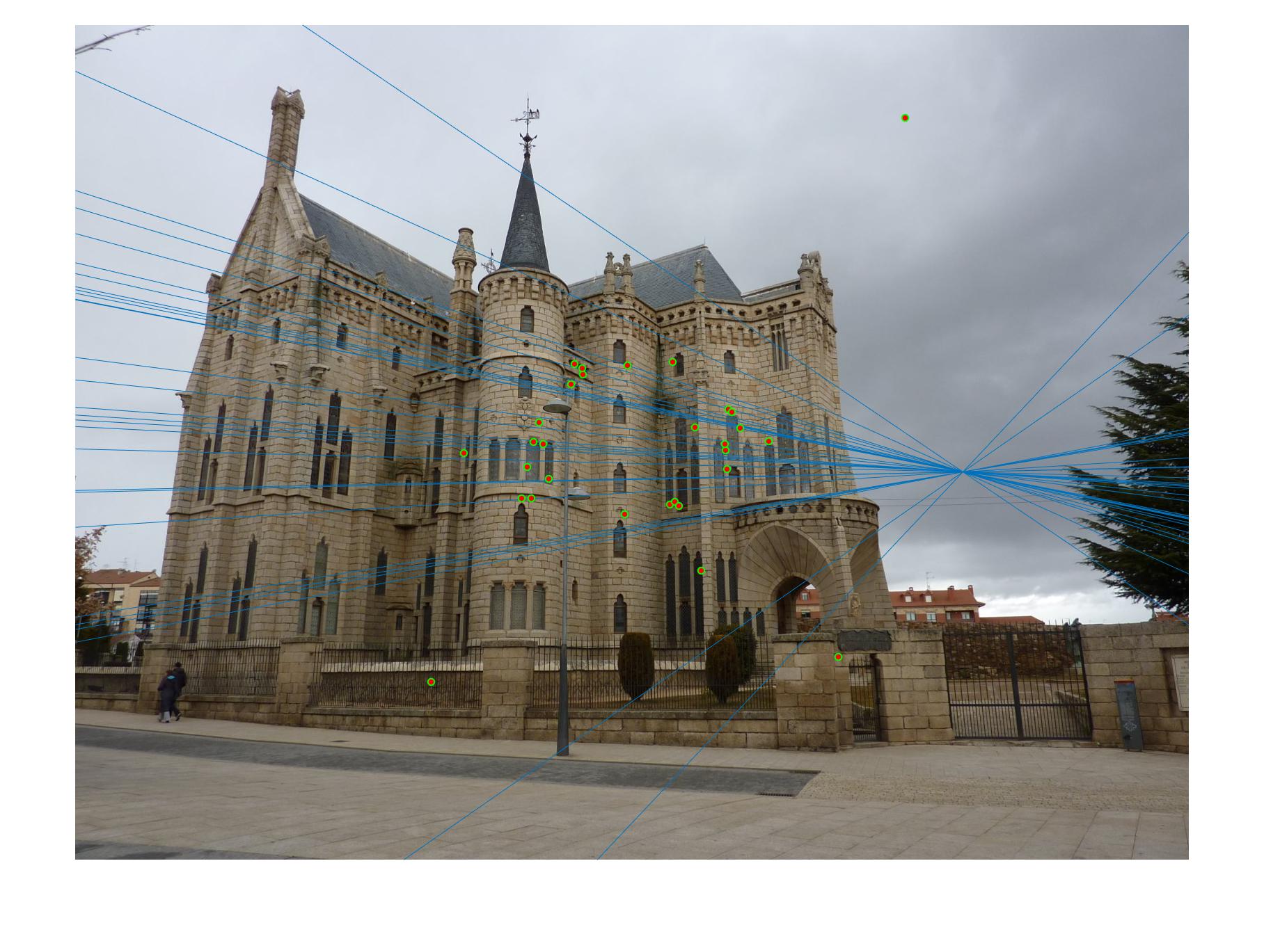
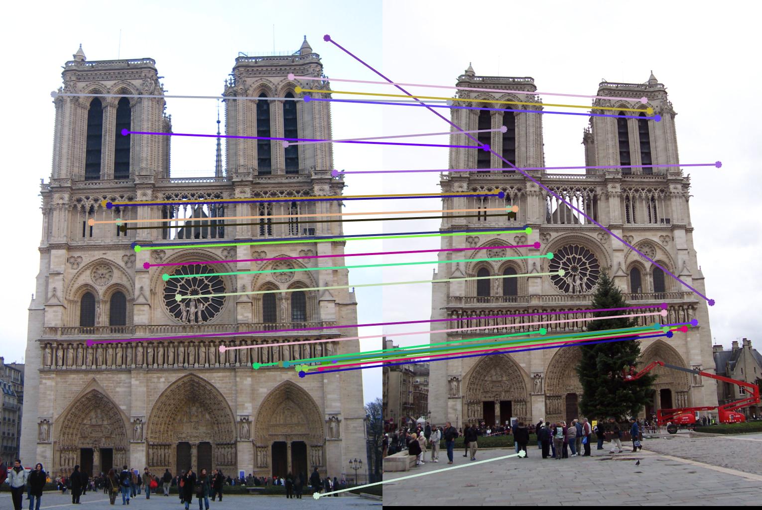
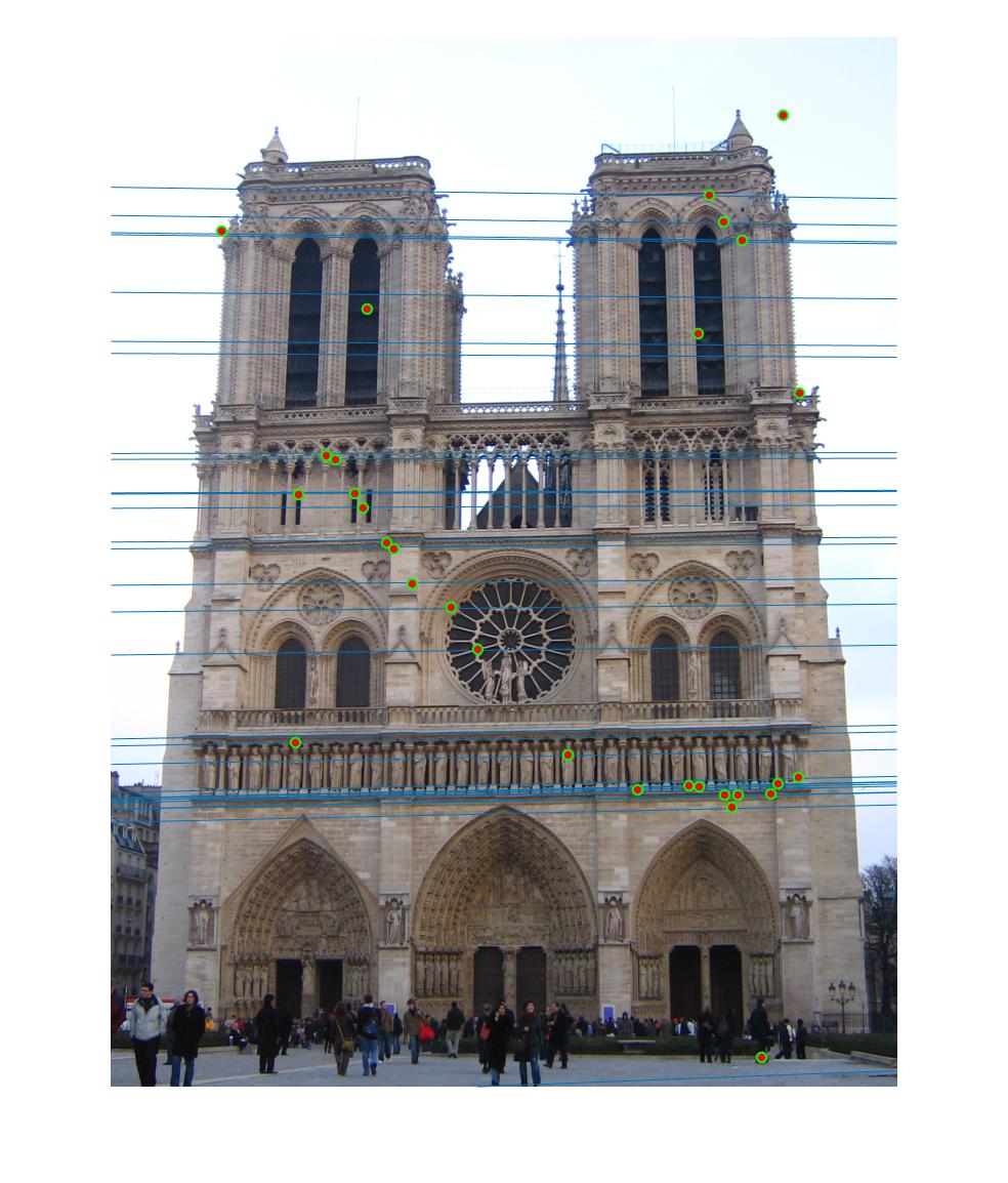
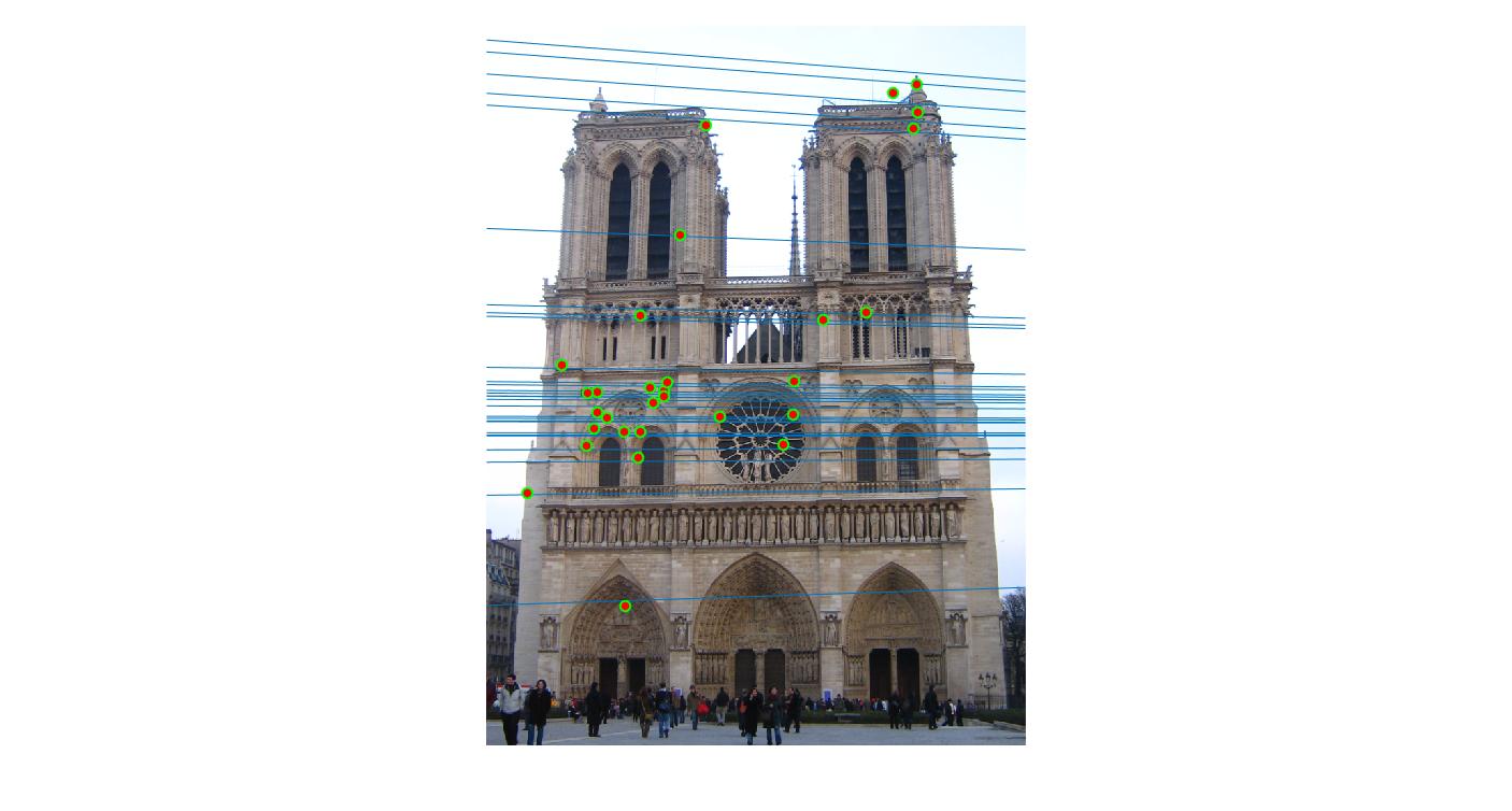
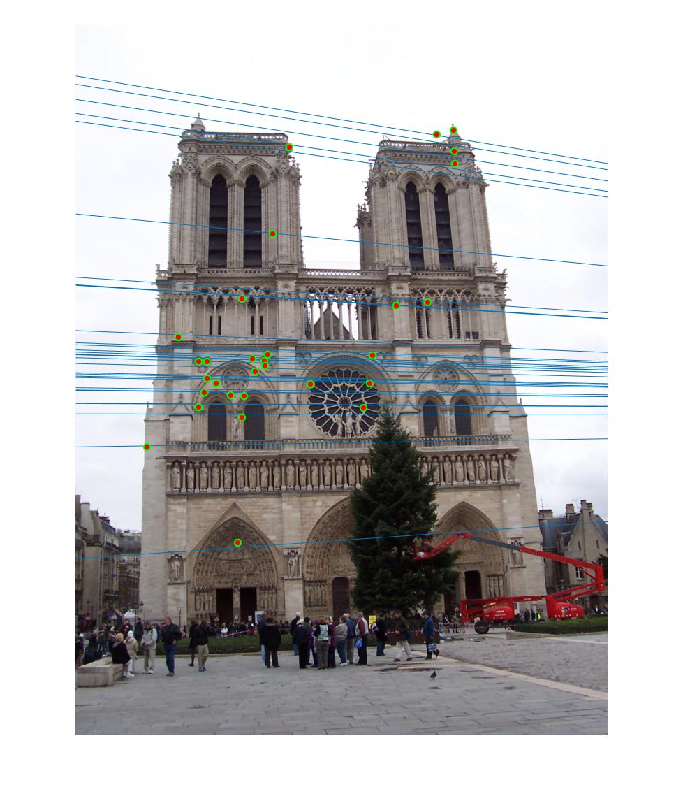
The F matrix corresponding to the maximum number of inliers is the best fitting model. The choice of threshold is very important to the algorithm. Here's how the results look for different values of threshold

Value in middle indicates threshold

0.01

0.05

0.1

0.2

0.3

As we can clearly see, increasing threshold decreases performance. In this case, threshold of around 0.05 seems to give the best fit.

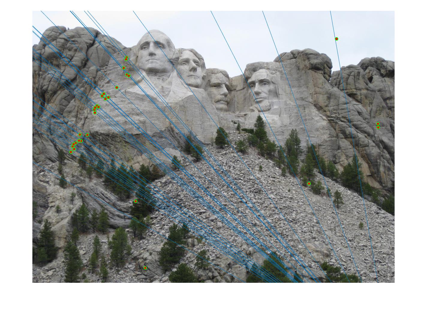
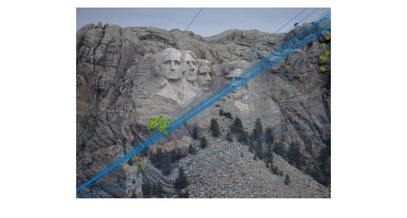
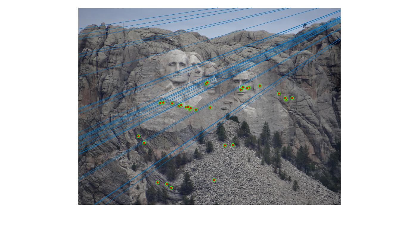
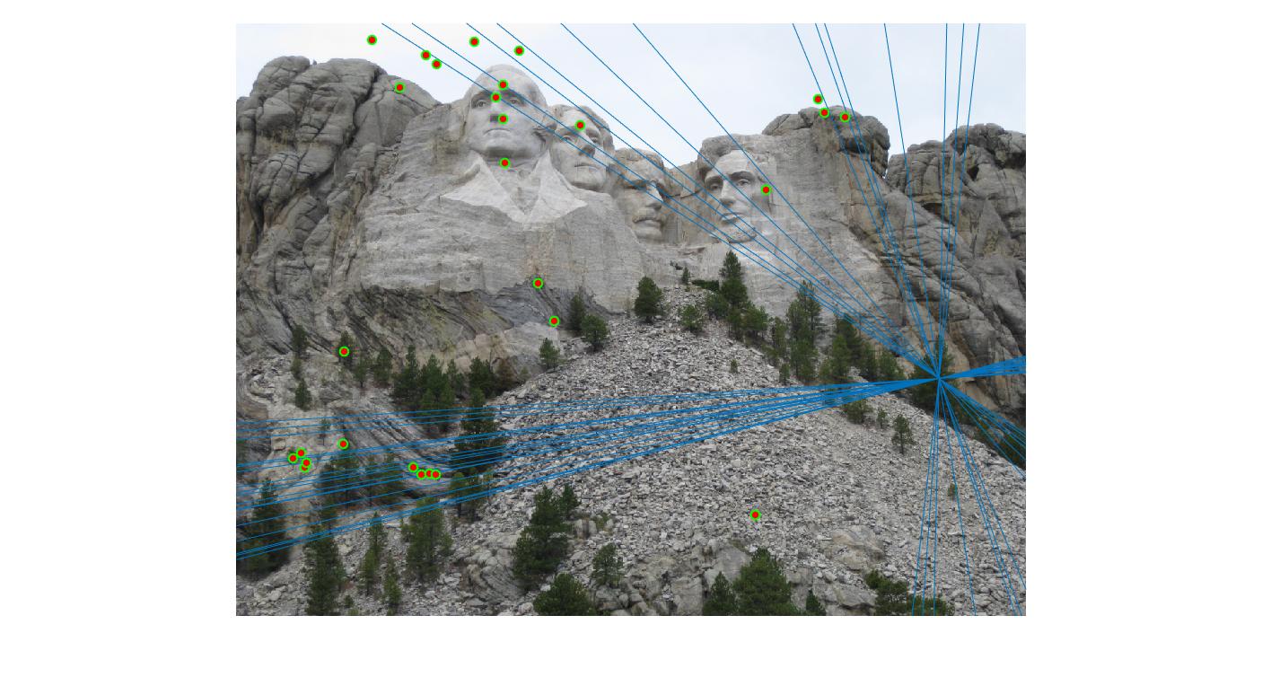
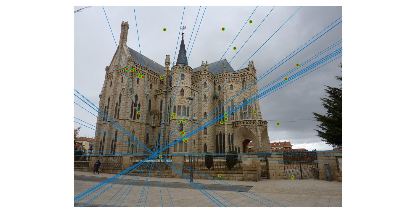
Since this is a random algorithm, it benefits from taking increased number of samples. Let's look at the response for different number of iterations of the rnsc algorithm.

Value in middle indicates number of iterations I ran the algorithm for. Threshold is set to 0.05

50

100

200

400

500

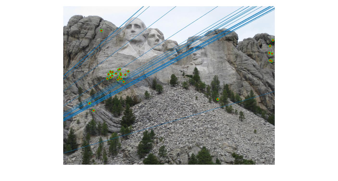
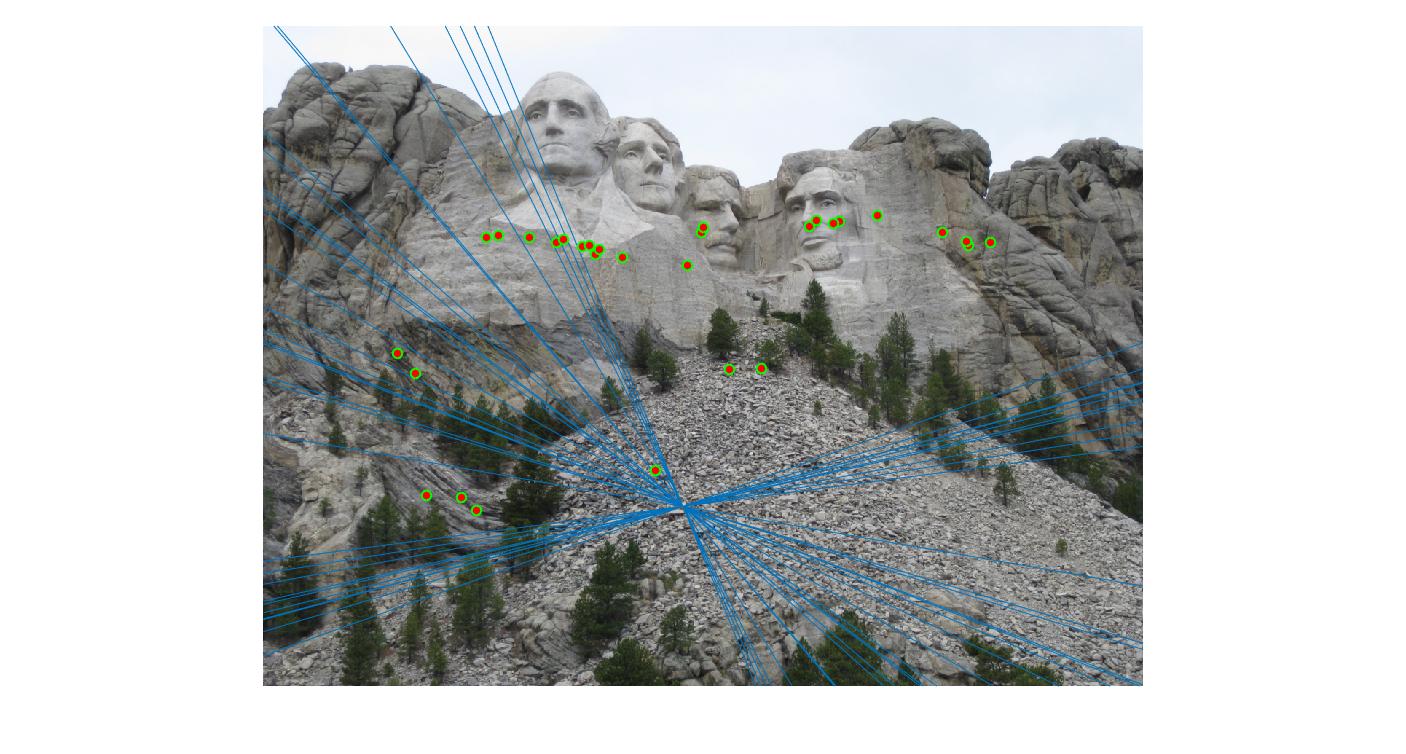
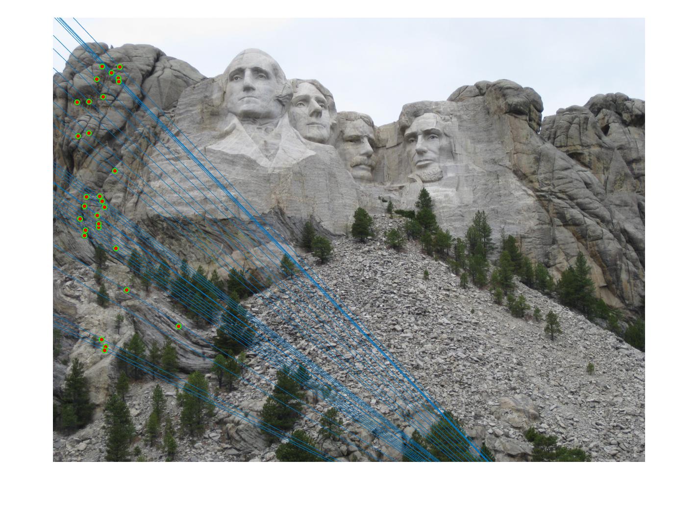
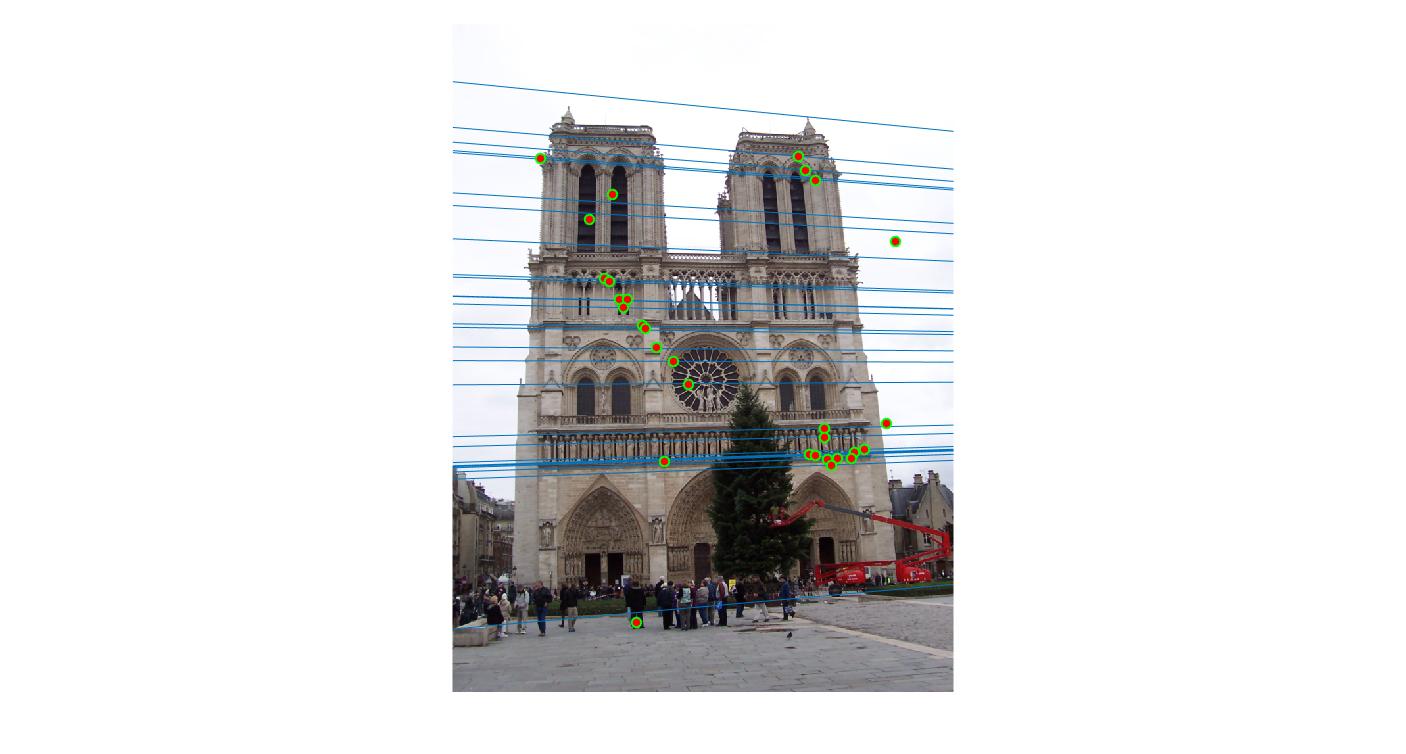
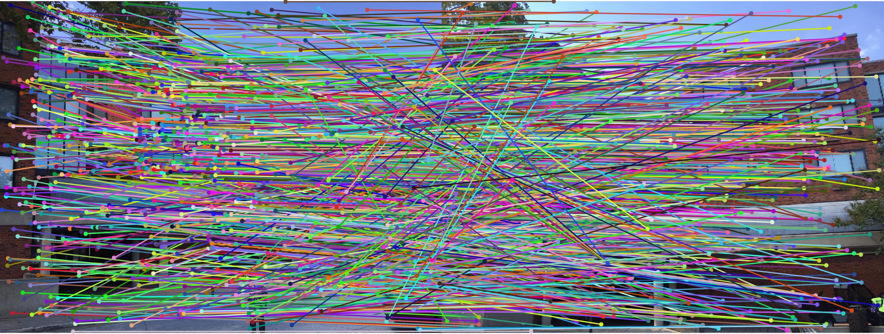
As can be clearly seen, running for a greater number of iterations gives better performance (fewer outliers). We can get bad results sometimes even for a high number of iterations as seen in the following case for N=700.

700

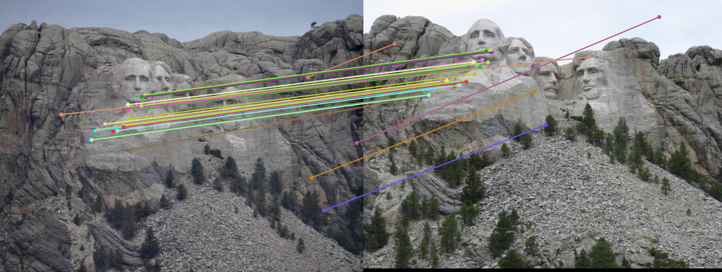
While there aren't any outliers, the model seems biased towards the left side of the image. Rerunning the algorithm, provides a different random start and should provide different results.

700 rerun

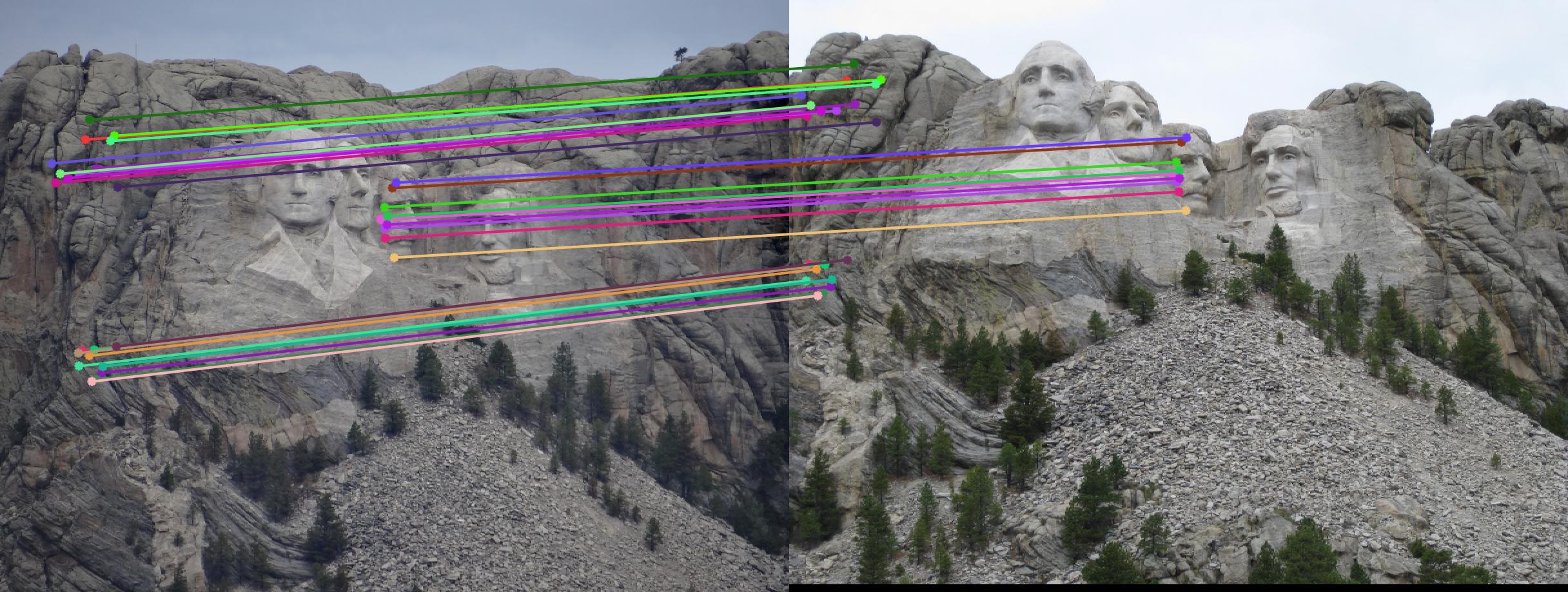
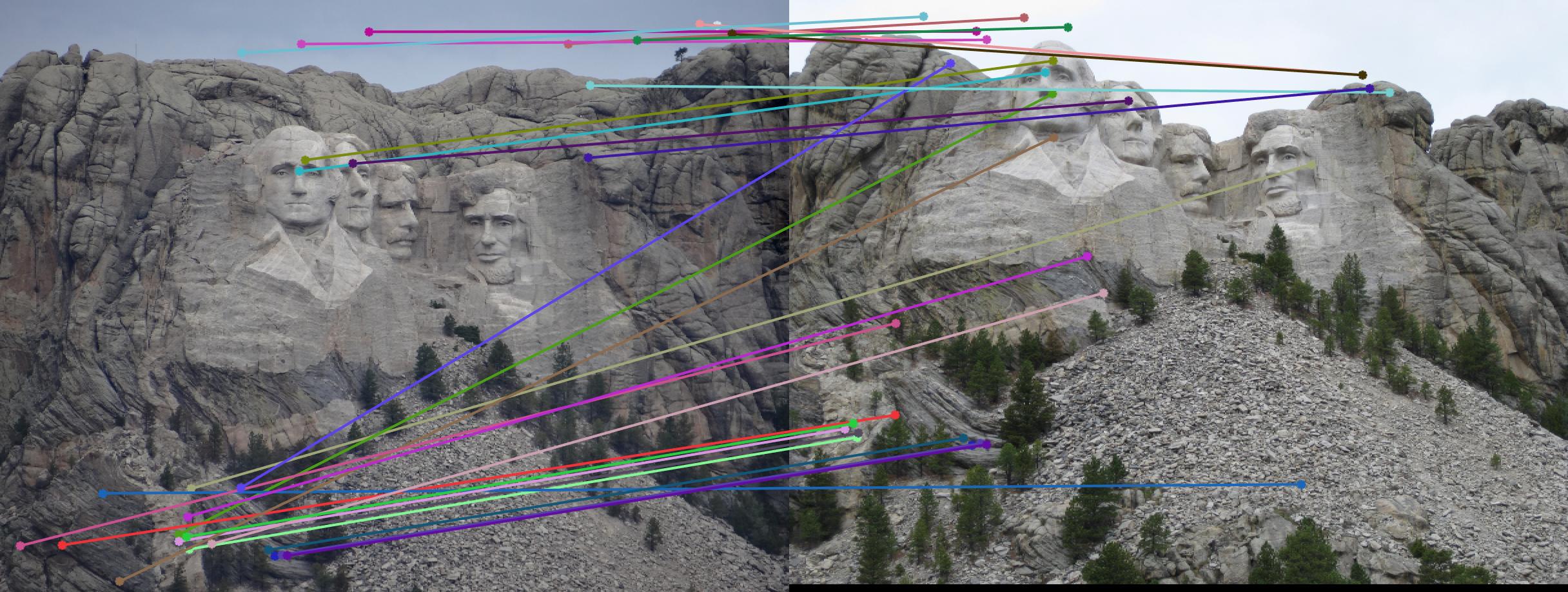
The points are now much more spreadout. A better technique would be to normalize the points first before fitting the model.

Extra credit - Normalization

Our estimate of the fundamental matrix can be improved by normalizing the points before finding the fundamental matrix. We translate the points to have zero mean, and scale them so that the average distance from origin is sqrt(2).

The matlab code is as follows:

        % Preconditioning
        xn = pa(1:2,:);
        N = size(xn,2);
        t = (1/N) * sum(xn,2);  % Centroid of coordinates
        xnc = bsxfun(@minus,xn,t);  % Subtract centroid
        dc = sqrt(sum(xnc.^2));  % Find average distance
        davg = (1/N)*sum(dc);
        s = sqrt(2)/davg;  % set scale so that average distance is sqrt(2)
        Ta = [s*eye(2), -s*t ; 0 0 1]; % set up normalization matrix
        pa = (Ta * pa)';  % Normalize points

        xn = pb(1:2,:);
        N = size(xn,2);
        t = (1/N) * sum(xn,2);
        xnc = bsxfun(@minus,xn,t);
        dc = sqrt(sum(xnc.^2));
        davg = (1/N)*sum(dc);
        s = sqrt(2)/davg;
        Tb = [s*eye(2), -s*t ; 0 0 1];
        pb = (Tb * pb)';

        ... Find F_matrix as before.

        % Postconditioning
        F_matrix = Ta' * F_matrix * Tb;
        

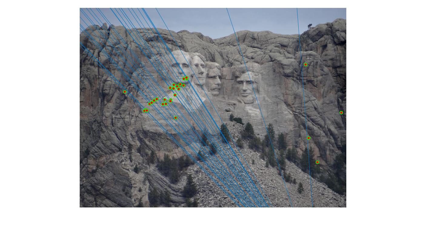
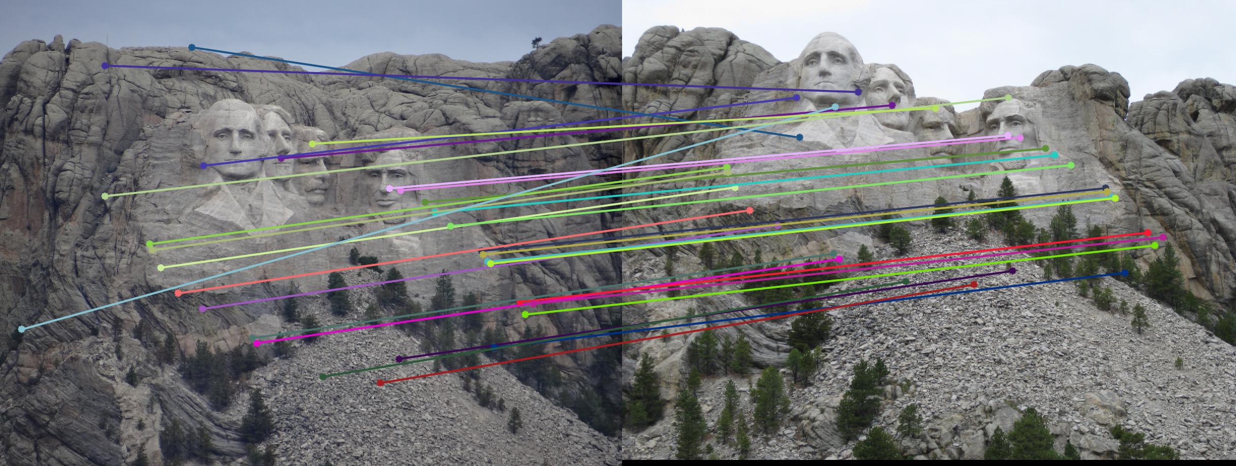
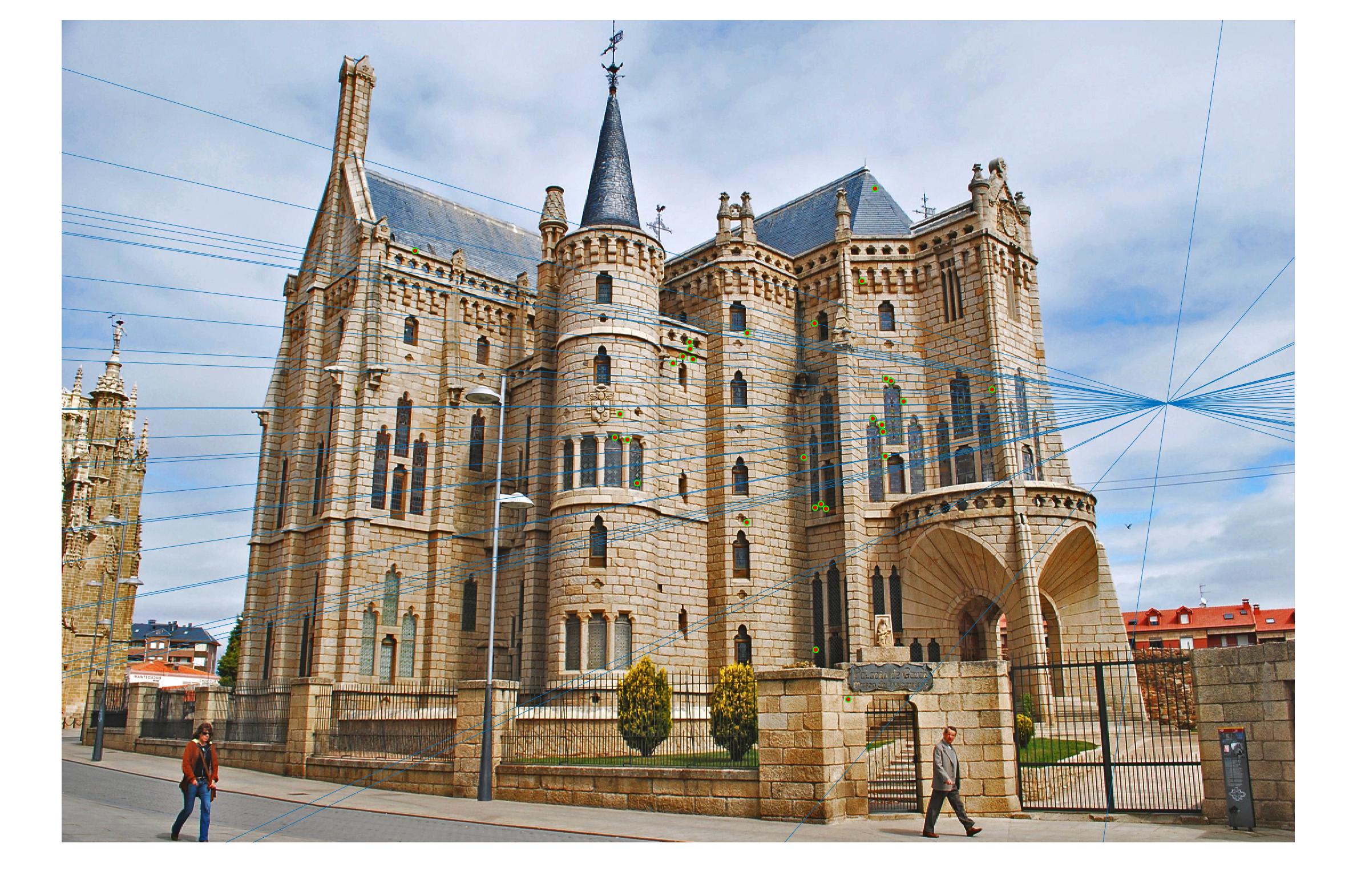
Normalizing makes a huge difference in the performance of our model. Let's take a look at the results. The text indicates the threshold and whether normalization was used or not. Different images need different thresholds.

0.17 False

0.17 True

0.09 False

0.09 True

0.07 False

0.07 True

As we can clearly see, normalization improves the performance of the model and reduces the number of outliers in the matches. This type of preconditioning is called Hartley's preconditioning.