Project 3 / Camera Calibration and Fundamental Matrix Estimation with RANSAC
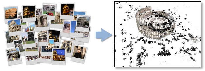
Structure from Multiple Image Views. Figure by Snavely et al.
The aim of this project is to understand the camera geometry and the scene geometry. The concept of mappping the 3D world coordinates to the 2D image coordinates is introduced. What are the epipolar lines, how the points of one image plane relate to the epipolar lines of other scene, how to estimate the fundamental matrix. We were given four images to test the results on:
- Mount Rushmore
- Notre Dame
- Episcopal Gaudi
- Woodruff Dorm
This project was divided into three parts:
Camera Projection Matrix:
The first step was to calculate the projection matrix. The most important part was to properly set up the matrix for computing the Singular Value Decomposition. It was important to keep in mind the number of variables and the corresponding equations required for setting up the regression. Then the value corresponding to the smallest singular value was taken and reshaped to give the final matrix. Using the same matrix the value of the camera centre was computed.
The projection matrix is:
[ 0.4583 -0.2947 -0.0140 0.0040 ;
-0.0509 -0.0546 -0.5411 -0.0524 ;
0.1090 0.1783 -0.0443 0.5968 ]
The total residual is: <0.0445>
The estimated location of camera is: <-1.5127, -2.3517, 0.2826>
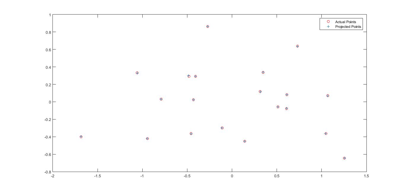
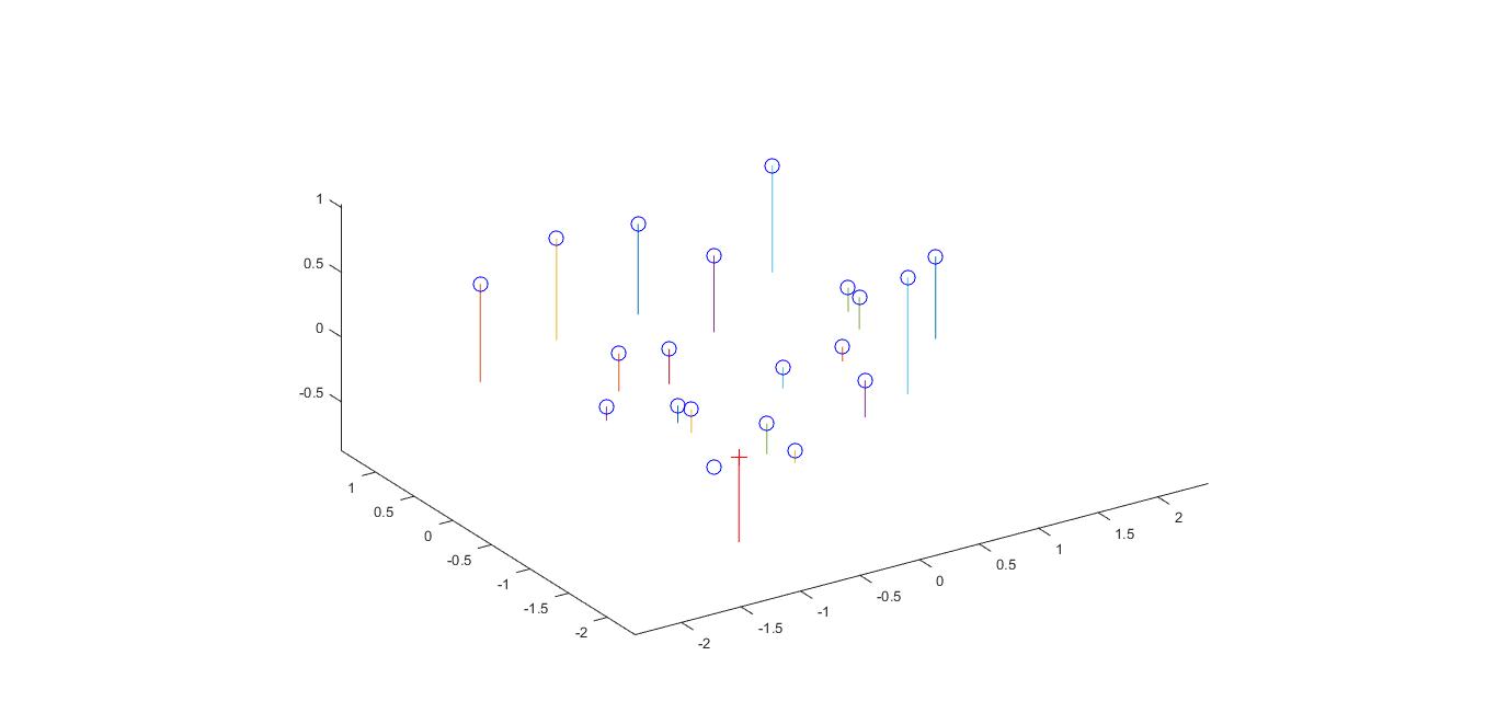
Image 1 Showing the position of the actual points and the points obtained after calculating them using the projected matrix. Image 2 Showing the computed camera centre. |
Fundamental Matrix Estimation:
Fundamental Matrix is used to relate the corresponding points in the stereo images. In this we just have one equation which is used to compute the 9 variables of the Fundamental Matrix, it was important to understand the structure of the equation and how to set it up like a linear regression problem. Once the matrix was computed, its least singular value was set to zero and using this matrix the Fundamental Matrix was computed. Whether the value of the Fundamental Matrix was correct or not was checked by plotting the epipolar lines using the matrix calculated. It was seen that although the majority of lines were passing through the marked points but many more were off by some amount.
The Fundamental Matrix for the Base Image Pair Pic_a and Pic_b
[ -5.36264198382955e-07 7.90364770857008e-06 -0.00188600204023535;
8.83539184115896e-06 1.21321685010684e-06 0.0172332901014492;
-0.000907382264407605 -0.0264234649922039 0.999500091906704 ]
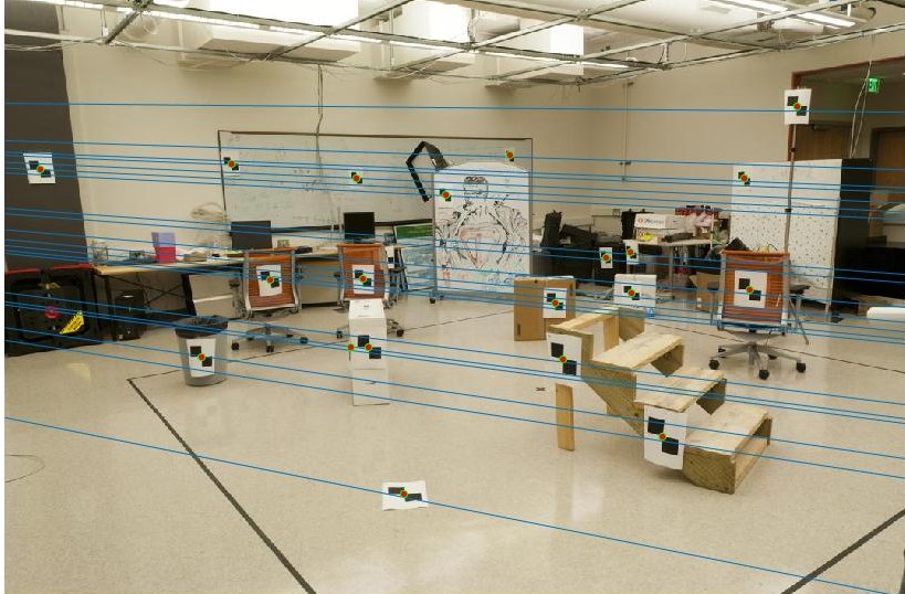
Image 1 Showing the epipolar lines calculated using the Fundamental Matrix for Base Image Pic_a. |
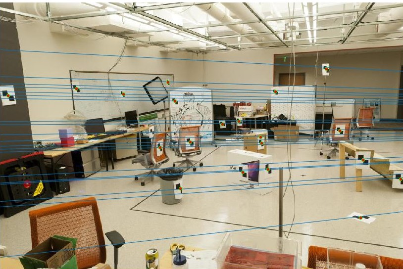
Image 2 Showing the epipolar lines calculated using the Fundamental Matrix for Base Image Pic_b. |
Fundamental Matrix using RANSAC:
First, the SIFT features were computed for both the images. The points were first randomly SAMPLED and eight points were picked up to calculate the Fundamental Matrix. This was further used to calculate the number of inliers and the matrix which gave the maximum number of inliers was the best Fundamental Matrix, but this estimate can be wrong, as the points can be coplanar or because of lens distortions. But this matrix is the best in removing the incorrect SIFT matches. For calculating the inliers, we calculated the distance metric. We set a cut-off value and all the points with the value less than this value were considered as inliers. We used the Fundamental Matrix constraint as a distance metric. We can also use the Sampson Error for the distance metric which is used to compute the distance of a point correspondence to the corresponding epipolar line of the point correspondence in the other image.
Analysis of the results
All the images were tested one by one by changing the number of iterations and the cut off value.
| Name of the Example | Number of iterations | Cut off Value used |
|---|---|---|
| Mount Rushmore | 1000 | 0.01 |
| Notre Dame | 1000 | 0.09 |
| Episcopal Gaudi | 3000 | 0.05 |
| Woodruff Dorm | 2000 | 0.07 |
Observations
Mount Rushmore
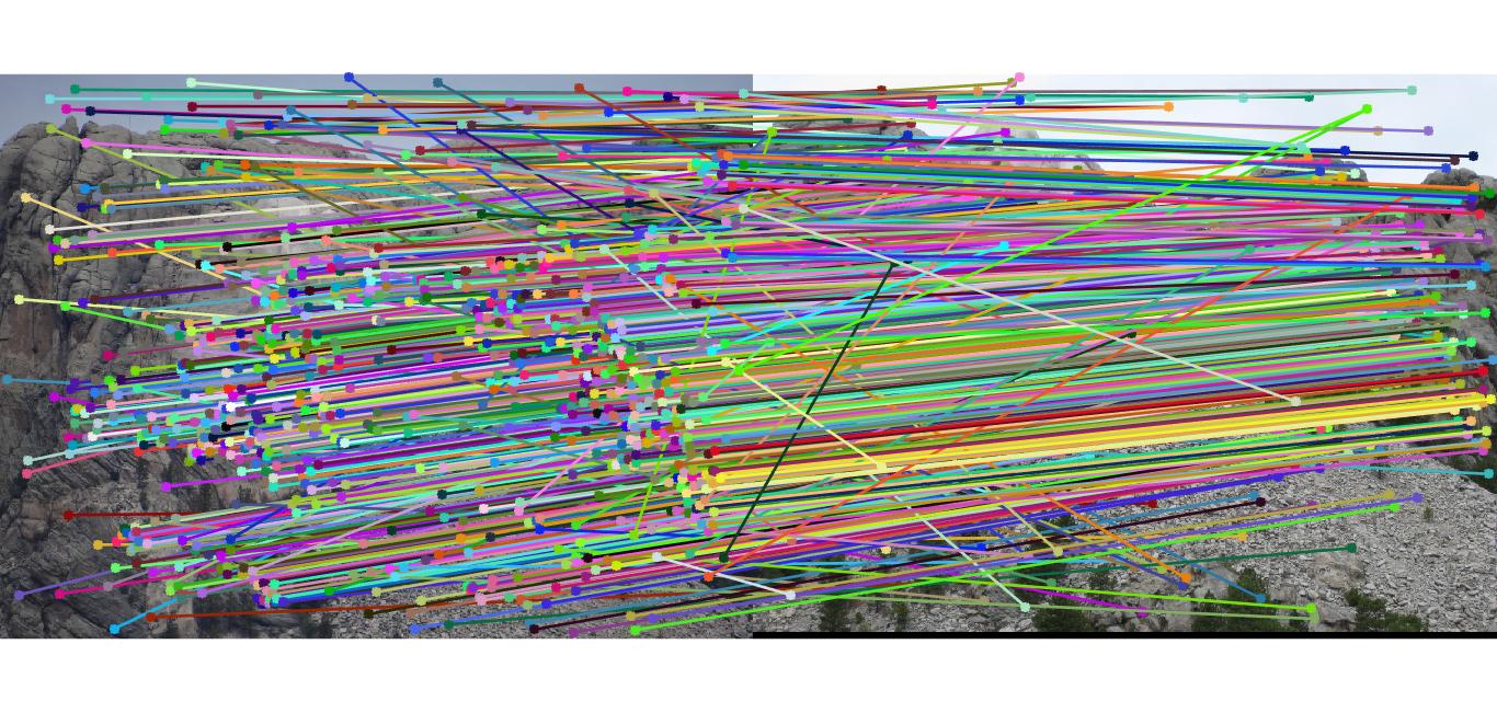
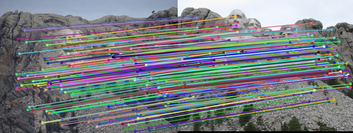
Image 1 showing the results of the correspondences before performing the RANSAC. Image 2 showing the results of the correspondences after performing the RANSAC. |
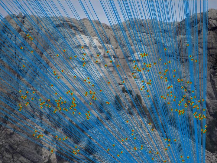
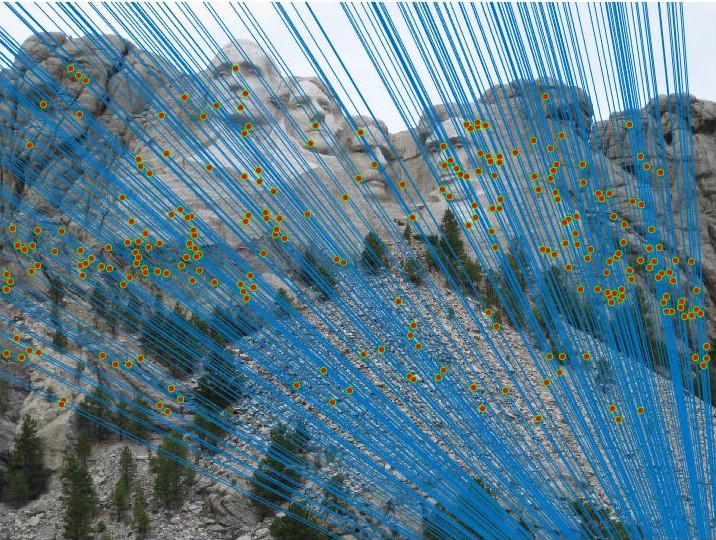
Image 3 showing the epipolar lines and Image 4 showing the epipolar lines in the same image but taken from a different angle. |
Notre Dame

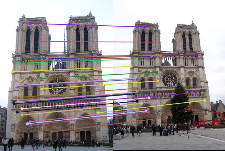
Image 1 showing the results of the correspondences before performing the RANSAC. Image 2 showing the results of the correspondences after performing the RANSAC. Only the top 30 matches are shown in this image. |
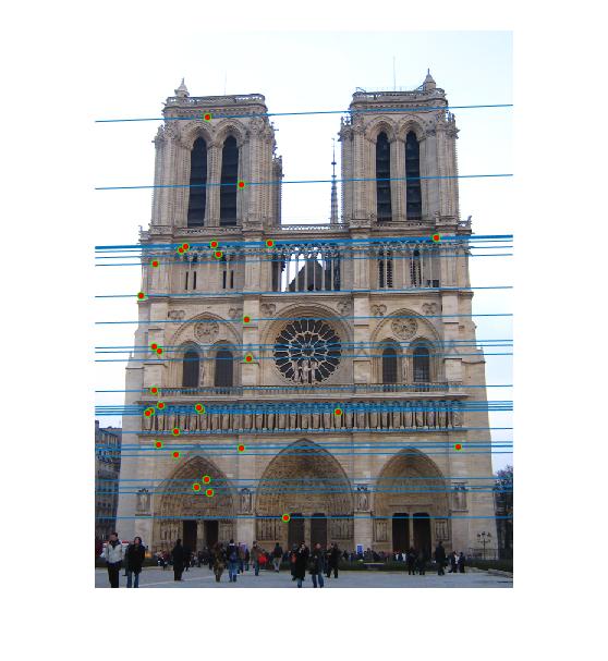
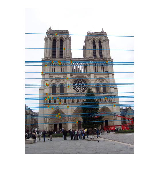
Image 3 showing the epipolar lines and Image 4 showing the epipolar lines in the same image but taken from a different angle. Only the epipolar lines corresponding to the top 30 inliers is shown in the image. |
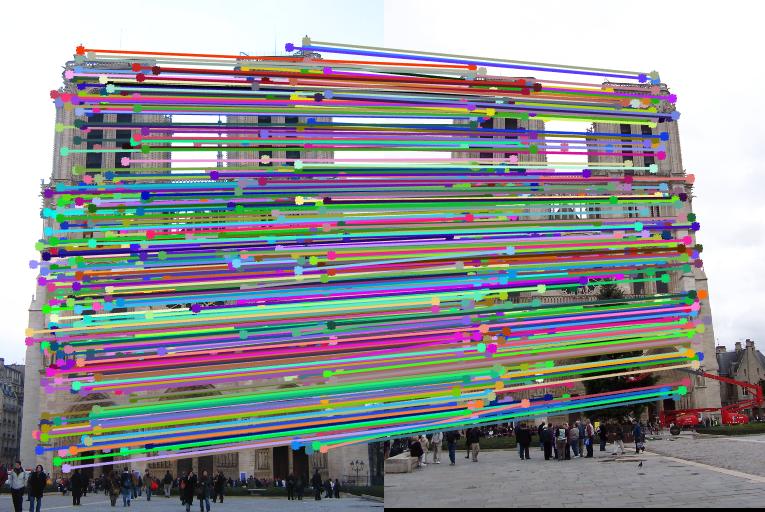
Image 1 showing the results of the correspondences before performing the RANSAC. Image 2 showing the results of the correspondences after performing the RANSAC. |
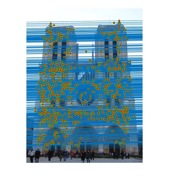
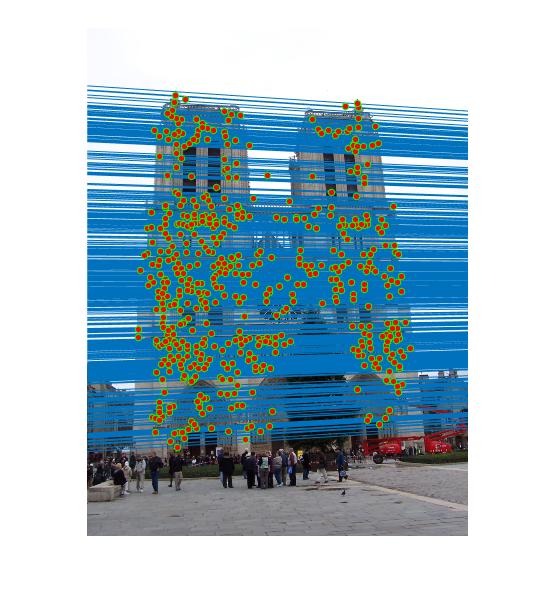
Image 3 showing the epipolar lines and Image 4 showing the epipolar lines in the same image but taken from a different angle. |
Episcopal Gaudi
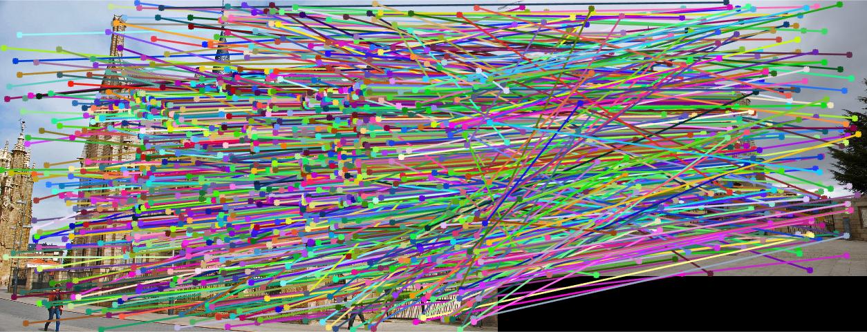
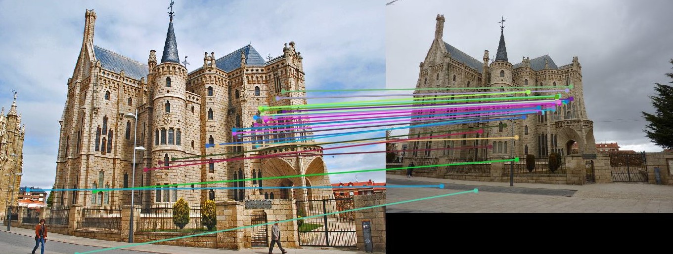
Image 1 showing the results of the correspondences before performing the RANSAC. Image 2 showing the results of the correspondences after performing the RANSAC. |
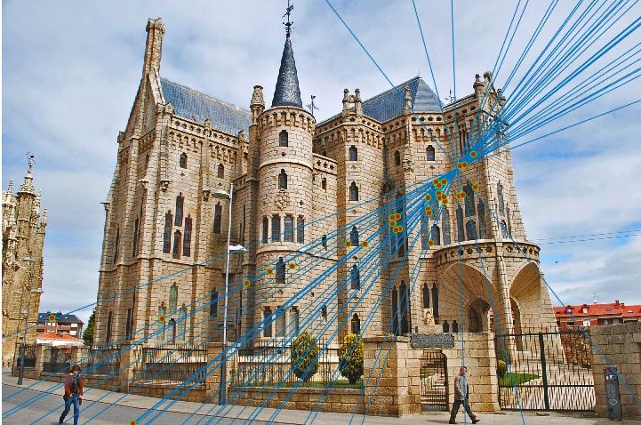
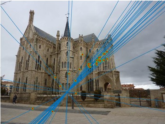
Image 3 showing the epipolar lines and Image 4 showing the epipolar lines in the same image but taken from a different angle. |
Woodruff Dorm
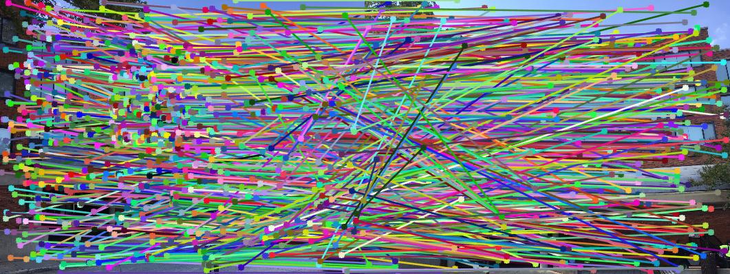
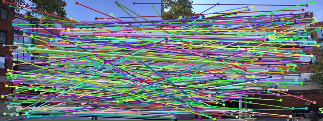
Image 1 showing the results of the correspondences before performing the RANSAC. Image 2 showing the results of the correspondences after performing the RANSAC. |
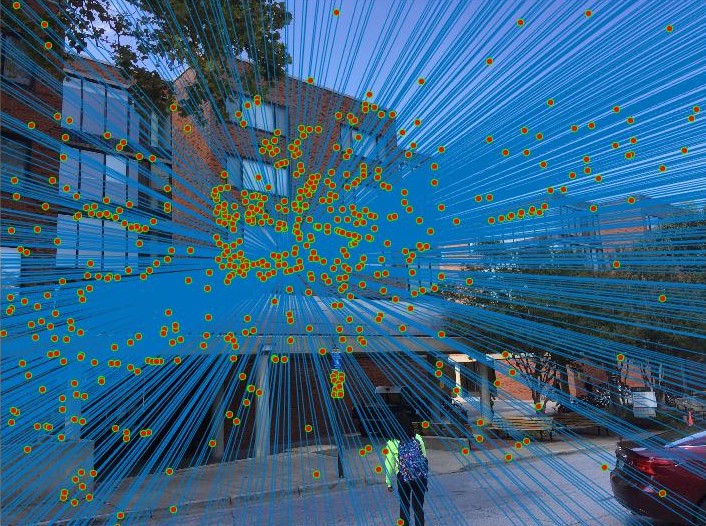
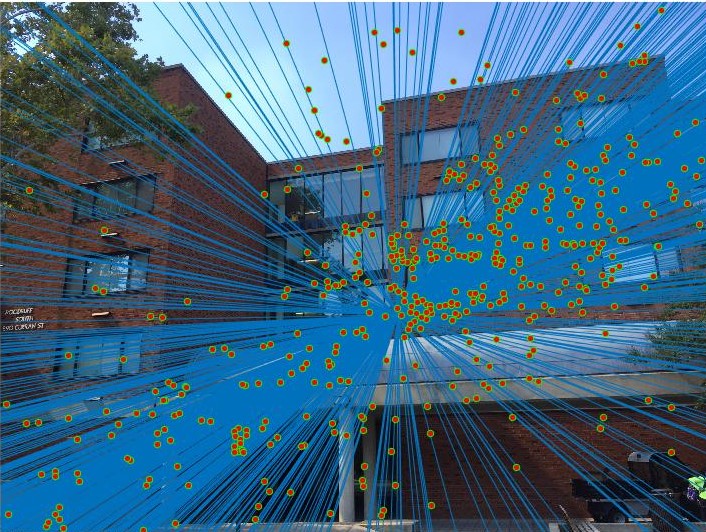
Image 3 showing the epipolar lines and Image 4 showing the epipolar lines in the same image but taken from a different angle. |
Some of the major issues faced were number of correspondences which were generated and that the epipolar lines were not exactly passing through the points.
Extra Credit
For resolving the second issue, the points were first normalized before using them for calculating the Fundamental Matrix. The normalization was performed by first calculating the mean of the coordinates and centring the image data at the origin. The scale factor was calculated by taking the average of the standard deviation of the coordinates u and v.Once the points were computed, the normalized points were used to calculate the Fundamental Matrix and smallest singular value was neglected. The the Fundamental Matrix was transformed back to the original coordinates.
The Fundamental Matrix for the Base Image Pair Pic_a and Pic_b after normalizing the coordinates:
[ -7.35602963795766e-06 9.65595699449298e-05 -0.0243607640894814 ;
6.06108182851019e-05 -1.84673297073191e-05 0.191366439044019 ;
0.000664772566212882 -0.259438462299607 5.22006218588355 ]
All the images were again tested one by one by changing the number of iterations and the cut off value after normalizing the points.
| Name of the Example | Number of iterations | Cut off Value used | No of Matching Features | Ratio of Inliers to Outliers |
|---|---|---|---|---|
| Mount Rushmore | 1000 | 0.01 | 825 | 207:618 |
| Notre Dame | 1000 | 0.09 | 851 | 568:283 |
| Episcopal Gaudi | 10000 | 0.05 | 1062 | 344:718 |
| Woodruff Dorm | 8000 | 0.07 | 887 | 268:619 |
Observations
Pic a and Pic b
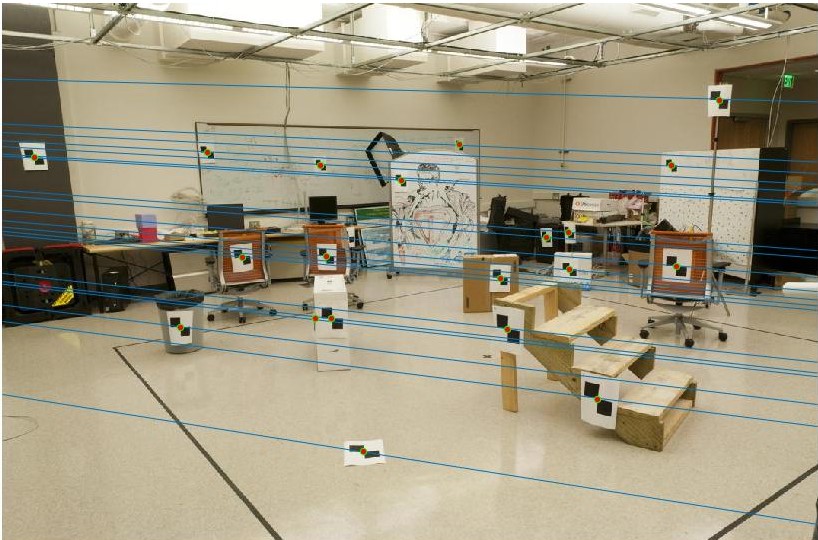
Image 1 showing the results of the Fundamental Matrix before and after normalization for Base Image Pic_a. |

Image 2 showing the results of the Fundamental Matrix before and after normalization for Base Image Pic_b. |
As can be seen the lines like the through the paper on the floor and the one at top of the ceiling did not pass through the makred points and were off by a margin. But in the image on the right, the results have improved.
Mount Rushmore
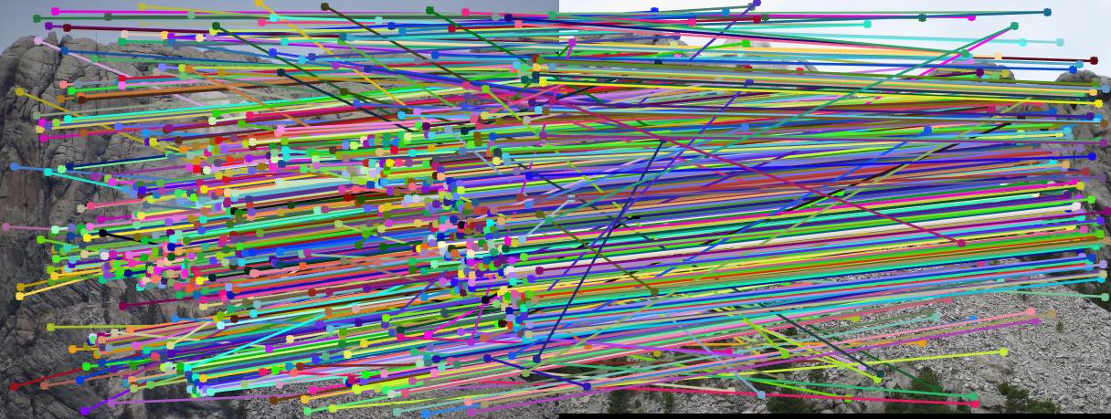
Image 1 showing the results of the correspondences before performing the RANSAC. Image 2 showing the results of the correspondences after performing the RANSAC. |
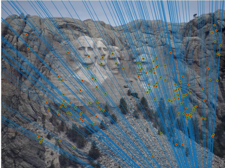
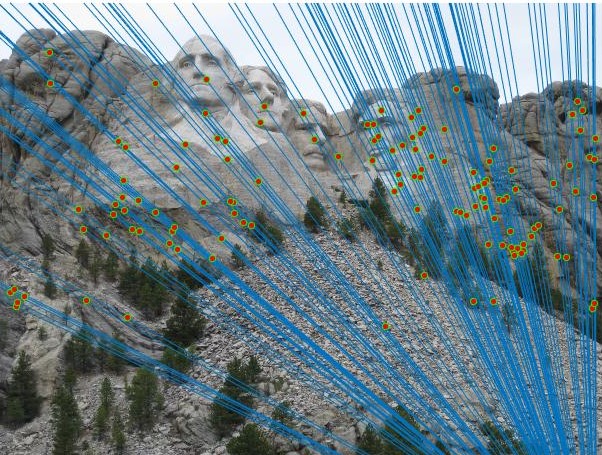
Image 3 showing the epipolar lines and Image 4 showing the epipolar lines in the same image but taken from a different angle. |
Notre Dame
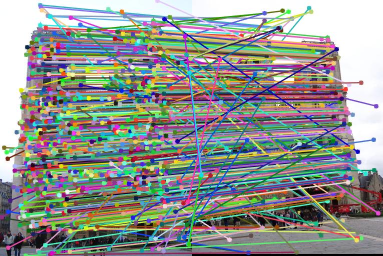
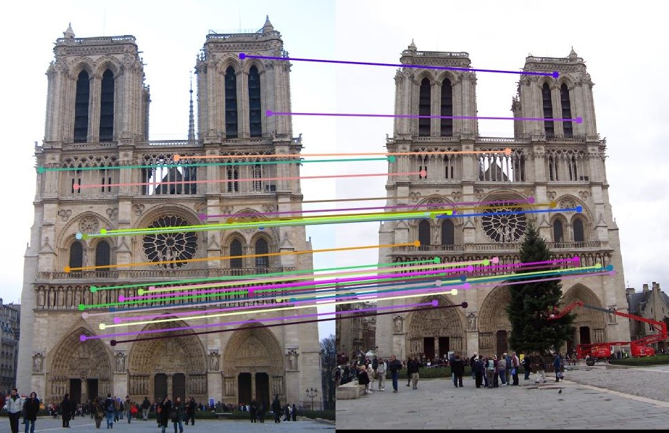
Image 1 showing the results of the correspondences before performing the RANSAC. Image 2 showing the results of the correspondences after performing the RANSAC. |
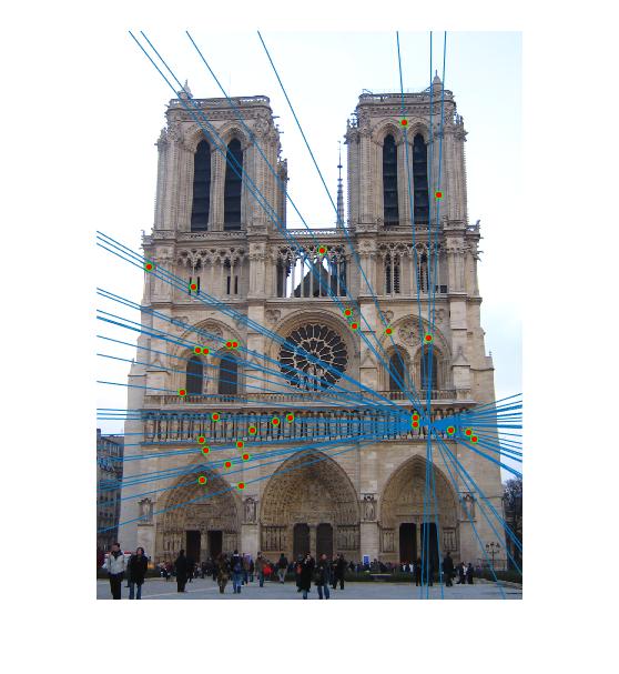
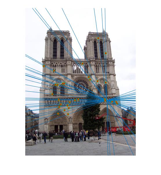
Image 3 showing the epipolar lines and Image 4 showing the epipolar lines in the same image but taken from a different angle. |
Episcopal Gaudi
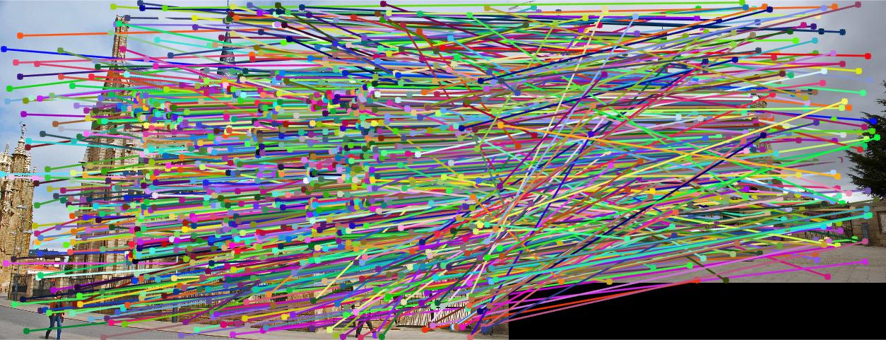
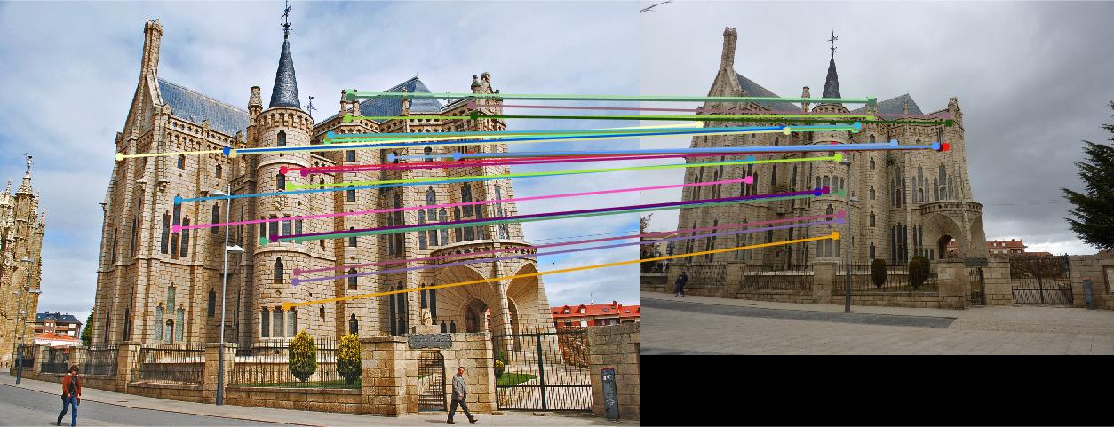
Image 1 showing the results of the correspondences before performing the RANSAC. Image 2 showing the results of the correspondences after performing the RANSAC. |
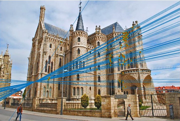
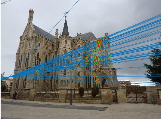
Image 3 showing the epipolar lines and Image 4 showing the epipolar lines in the same image but taken from a different angle. |
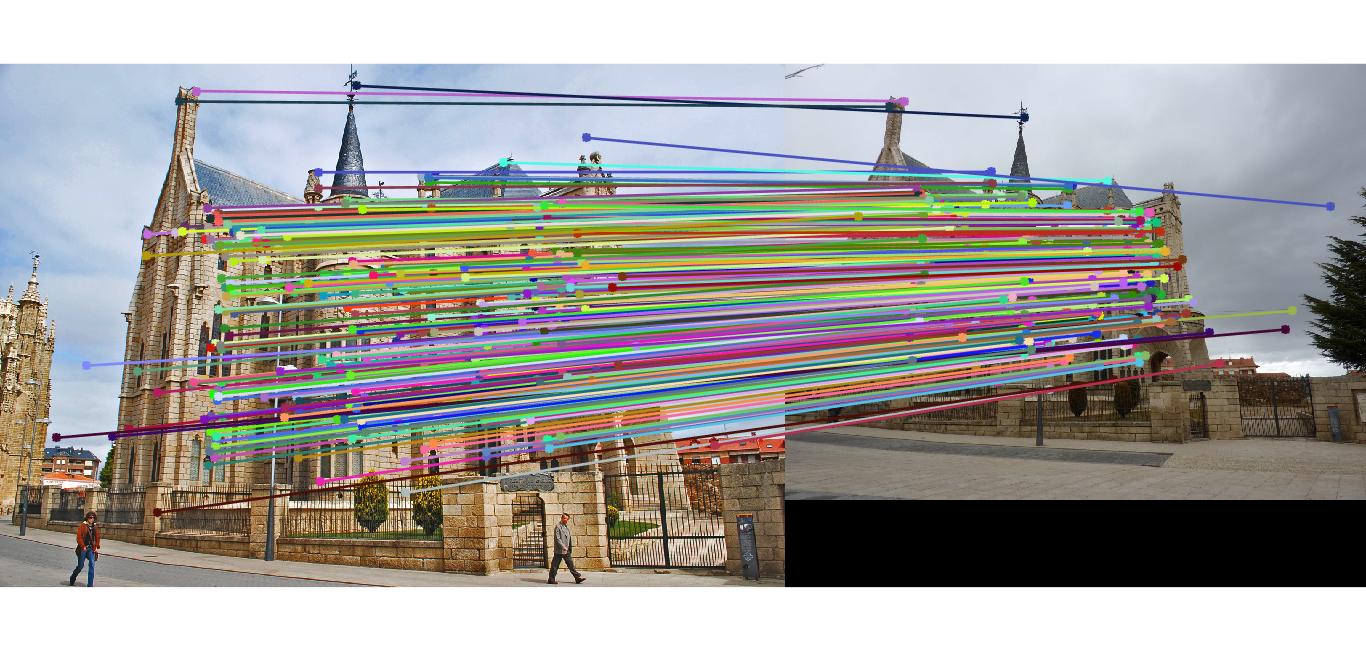
Image 1 showing the results of the correspondences before performing the RANSAC. Image 2 showing the results of the correspondences after performing the RANSAC. This was run for 10000 iterations of RANSAC, thus giving dense correspondences. |
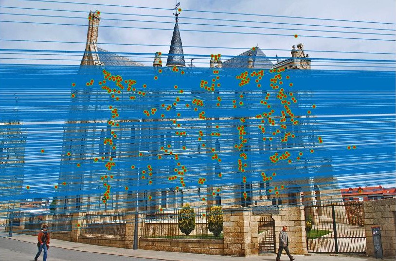
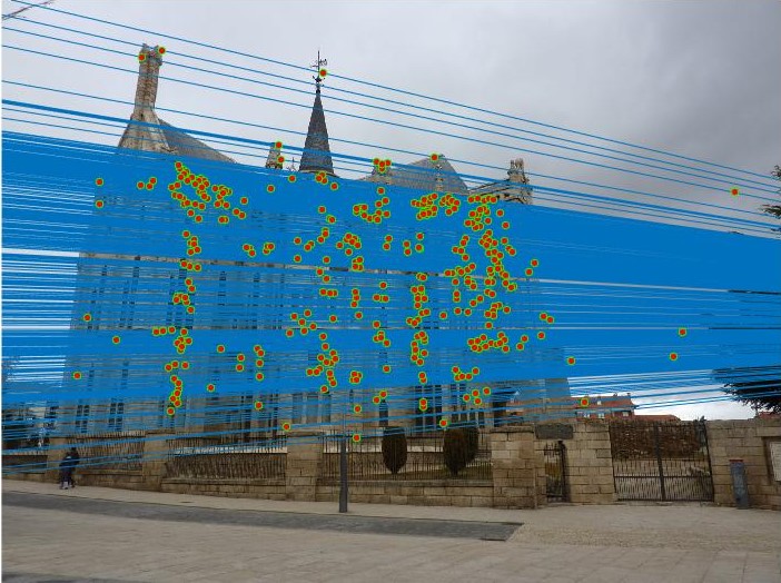
Image 3 showing the epipolar lines and Image 4 showing the epipolar lines in the same image but taken from a different angle. This was run for 10000 iterations of RANSAC, thus giving dense epipolar lines. |
Woodruff Dorm
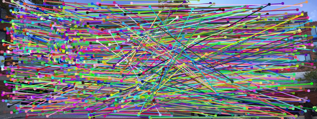
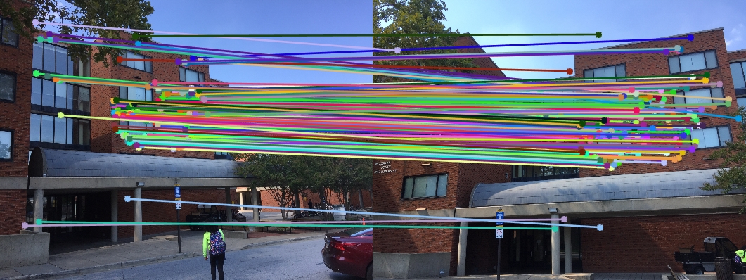
Image 1 showing the results of the correspondences before performing the RANSAC. Image 2 showing the results of the correspondences after performing the RANSAC. |
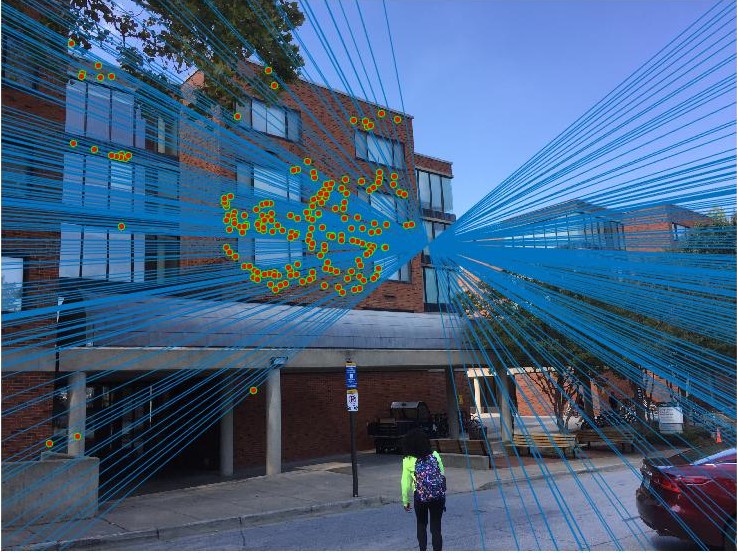
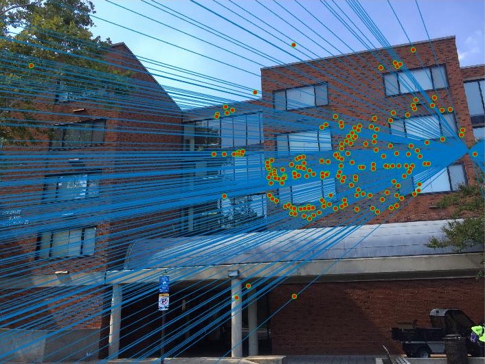
Image 3 showing the epipolar lines and Image 4 showing the epipolar lines in the same image but taken from a different angle. |
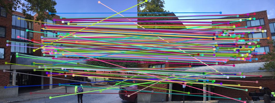
Image 1 showing the results of the correspondences before performing the RANSAC. Image 2 showing the results of the correspondences after performing the RANSAC. This was run for 10000 iterations of RANSAC. |
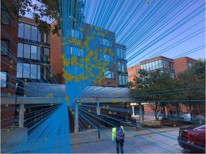
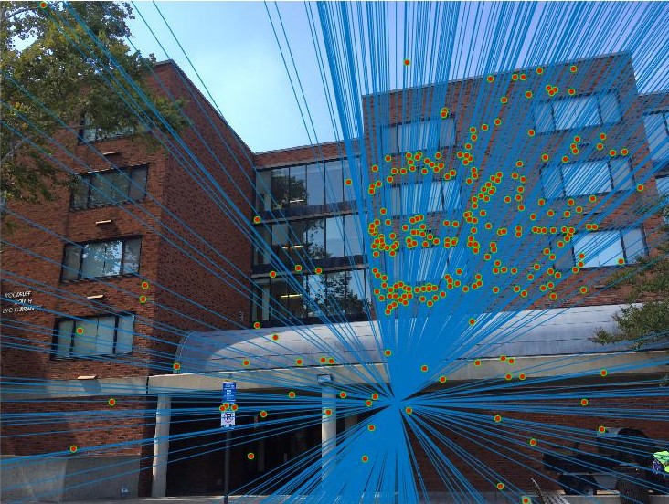
Image 3 showing the epipolar lines and Image 4 showing the epipolar lines in the same image but taken from a different angle. This was run for 10000 iterations. |
Conclusion
The Camera centre, projection matrix and the Fundamental MAtrix with the application of RANSAC were succesfully implemented. The correspondences and the epipolar lines were obtained.