Project 3 / Camera Calibration and Fundamental Matrix Estimation with RANSAC
In short, this project is an opportunity for us to explore how we can take images and allow a computer to visualize them in a 3D space. This is useful when comparing two images of the same object taken from different angles and serves as an expansion to the work that we did in the previous project with the SIFT descriptors. There are three major components to this project that we will examine one by one.
- The Camera Projection Matrix: predicting where the camera's location was to create the image
- The Fundamental Matrix: Mapping points from one image to another
- RANSAC Implementation: Using the Fundamental Matrix to eliminate spurious SIFT matches
Section 1 is where we deal with the conversion between 2D and 3D as we go through the implementation of calculate_projection_matrix.m and compute_camera_center.m. The logic discussed here is what allows us to predict where the camera center was located to take a particular image. Section 2 is where we deal with the conversion between coordinate points of two different images through the implementation of estimate_fundamental_matrix.m. The logic discussed here is what allows us to use a set of coordinate points from each of the two different images of the same object (the inputs are points matched via SIFT later on in the project) to guess what the fundamental matrix must have been to convert between the two sets. Finally, Section 3 is where we use the logic from Section 2 to assist in weeding out spurious SIFT matches through the implementation of ransac_fundamental_matrix.m. The logic discussed here is what allows us to improve the accuracy of our feature matching between two images via RANSAC. It has a dependency on estimate_fundamental_matrix.m, which will be examined in our discussion for this section. Furthermore, extra credit was pursued with normalization of the fundamental matrix, which will be examined here as well.
The Camera Projection Matrix
In this section, we deal with the projection matrix, a means of mathematically determining the likely location of the camera center that was necessary to take a picture. For us to achieve this, we are given a corresponding set of 2D points and 3D points in which for any particular index i, 2D(i) maps to 3D(i). Given this, the approach is fairly simple: we first use these corresponding points to create a set of linear combinations. These linear combinations will have 12 variables involved, one for each of the values in the projection matrix we are calculating for in the end. The code snippet below describes what we are doing (note that the elipses/line breaks are mainly there for readability and that each of the linear combinations are added as one row at a time).
  num_pairs = size(Points_2D, 1);
  pair_combinations = zeros(2*num_pairs, 12);
  for i = 1:num_pairs
      x = Points_3D(i, 1);
      y = Points_3D(i, 2);
      z = Points_3D(i, 3);
      u = Points_2D(i, 1);
      v = Points_2D(i, 2);
      %m_{11}X + m_{12}Y + m_{13}Z + m_{14} - m_{31}uX - m_{32}uY - m_{33}uZ - m_{34}u
      %m_{21}X + m_{22}Y + m_{23}Z + m_{24} - m_{31}vX - m_{32}vY - m_{33}vZ - m_{34}v
      pair_combinations(2*i-1, :) = [x, y, z, 1, ...
                                     0, 0, 0, 0, ...
                                     -u*x, -u*y, -u*z, -u];
      pair_combinations(2*i, :) = [0, 0, 0, 0, ...
                                   x, y, z, 1, ...
                                   -v*x, -v*y, -v*z, -v];
  end

  [~, ~, V] = svd(pair_combinations);
The comments above the lines where we are adding to our linear combinations
more or less describe the equation we are representing. How we derive these expressions
is explained on the project website and can be reviewed there, but the general idea
is we are considering how given the values within the projection matrix, the 3D
points would be mapped to the 2D points in a particular way and expanding out
the matrix multiplication operation to reach it. With that said, note the call to
svd() after we have gone through the entire set points. Our input is the set of
linear combinations and here we are essentially performing a singular value decomposition
to determine what each of the values within the projection matrix are meant to be.
We don't care about the first two matrices returned, just the column vector V because
that contains all the values (the first two matrices are part of the result of the decomposition
to maintain the result's overall identity with the matrix passed in. For more details,
review what a singular value decomposition is.). Since V is just a row vector,
our final step is to make a 3x4 projection matrix M and iterate through V and
place the value in the appropriate part of M, going left to right and moving
on to the next row as necessary. In the context of the pictures tested for this part of
the project, I merely had to multiply the values from V by a factor of -1 as I
stored them into the resulting projection matrix to get similar numbers to those
mentioned on the project website.
As for computing the camera center, this is more or less as simple as splitting
the camera projection matrix into two sections: a 3x3 from the first 3 columns (which
we proceed to negate and invert) and a 1x3 from the last column. We multiply the two components
together to determine the camera center.
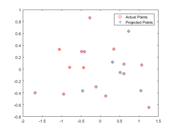
Now that we've gone through the theory behind this section's implementation,
let's examine its results. Going from left to right, the first image checks
the projection matrix that was calculated in calculate_projection_matrix.m and
makes sure that it was calculated correctly. We can be sure that it was generally
correct in this particular case because the projected points are more or less
at the same location as the actual points, as demonstrated by the blue +'s and
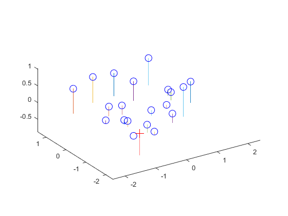
red circles, respectively. The second image shows us the estimated camera center
location, as represented by the red cross on the image. It's clear that the
estimated camera location would be adequate to view all the other points in the
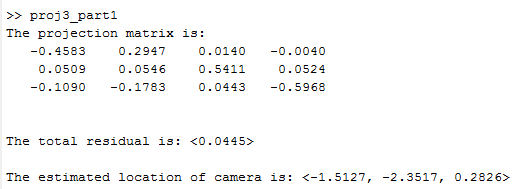
graph. Finally, the third image is a terminal screenshot of running proj_part1.m,
and the result shown is consistently achieved. Therefore, the estimated location
of the camera center was determined to be <-1.5127, -2.3517, 0.2826>.
|
The Fundamental Matrix
So we can determine where the camera was located, great. But what if we want to figure out how to map 2D points of one image to 2D points of another from a different angle, rather than map 2D to 3D? This is where the fundamental matrix comes into play. Here, we follow similar logic to that described in the previous section, and generate the matrix through the use of many linear combinations. A snippet of this section is presented below.
  num_combinations = size(Points_a, 1);
  fundamental_combinations = zeros(num_combinations, 9);
  for i=1:num_combinations
     %a = (u, v)
     a_u = Points_a(i, 1);
     a_v = Points_a(i, 2);
     %b = (u', v')
     b_u = Points_b(i, 1);
     b_v = Points_b(i, 2);
     %f11*u*u'+f12*v*u'+f13*u'+f21*u*v'+f22*v*v'+f23*v'+f31*u+f32*v+f33
     fundamental_combinations(i, :) = [a_u*b_u, a_v*b_u, b_u, ...
                                       a_u*b_v, a_v*b_v, b_v, ...
                                       a_u, a_v, 1];

  end

  [~, ~, V] = svd(fundamental_combinations);
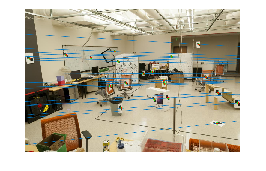
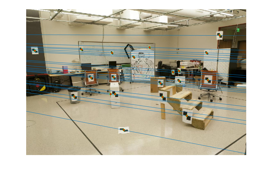
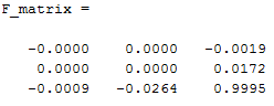
Using the same idea in the previous section: we use the values in the column vector V to generate the fundamental matrix. Fairly simple. With this in mind, we can use our estimated fundamental matrix to graph epipolar lines along our input images to validate our estimate. As we can see among the first two images in the table below, the epipolar lines seem to match fine, as we see them moving straight along each of the particular points we were checking for and it's easy to visualize the relationship between the two as rotating the view to the right as the transition between the first image and the second one. Finally, the third image is the matlab output for the estimation for the unnormalized fundamental matrix for the two input images pic_a.jpg and pic_b.jpg. Normalization of the fundamental matrix will be discussed later on into the next section.
|
RANSAC Implementation
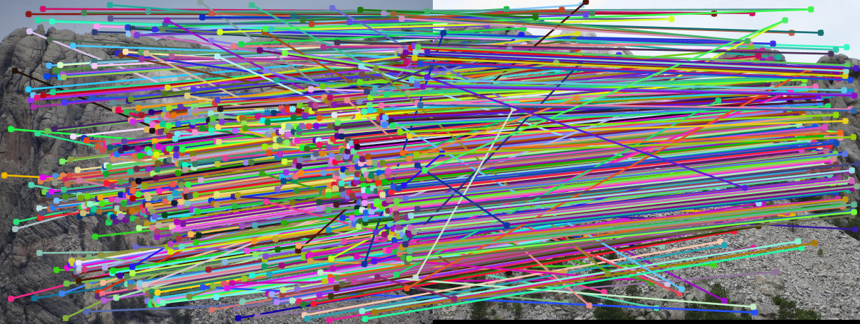
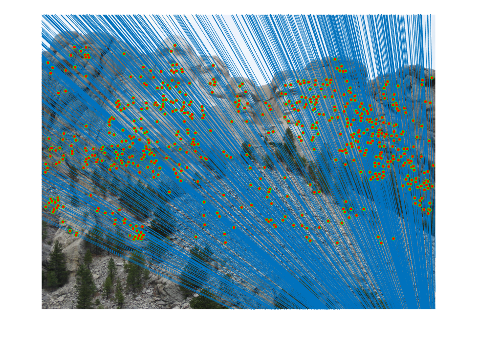
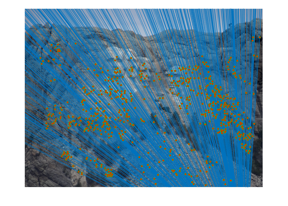
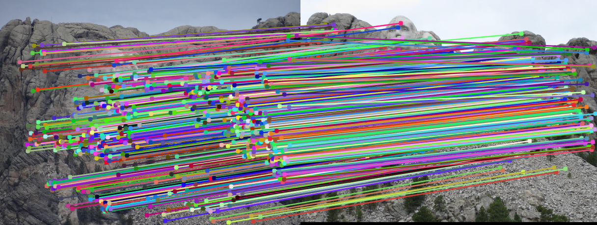
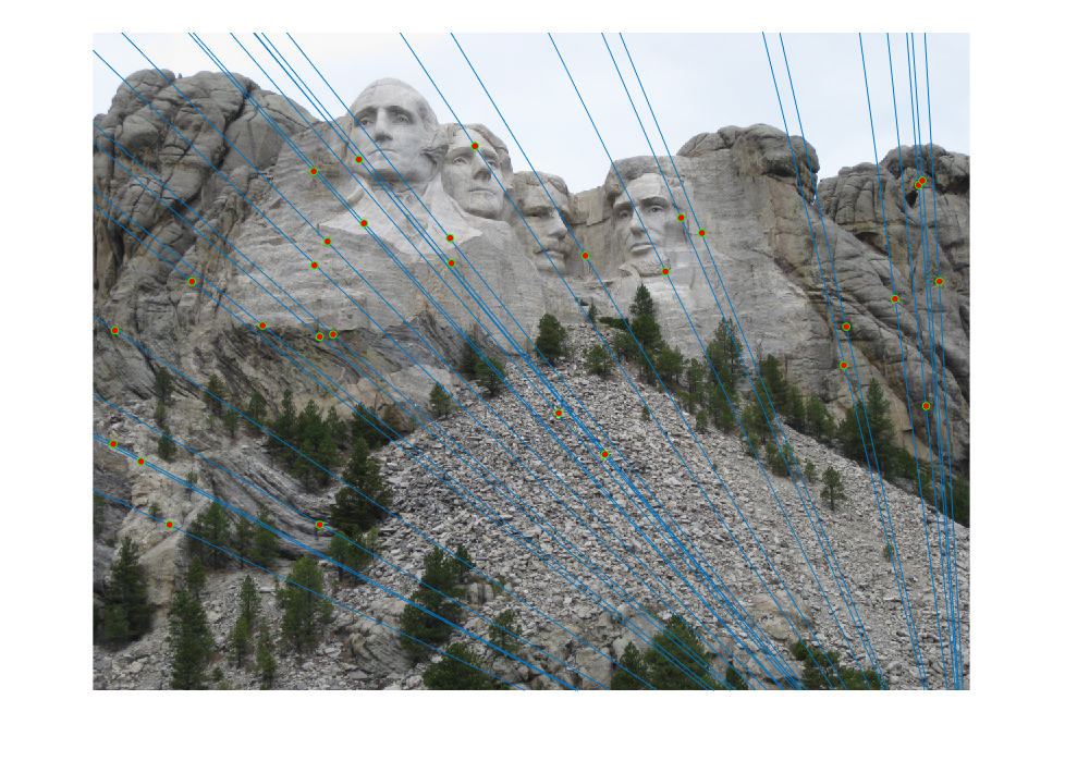
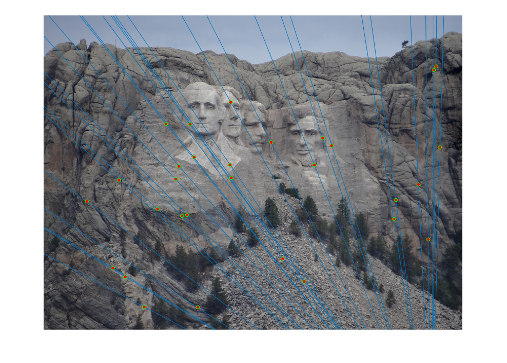
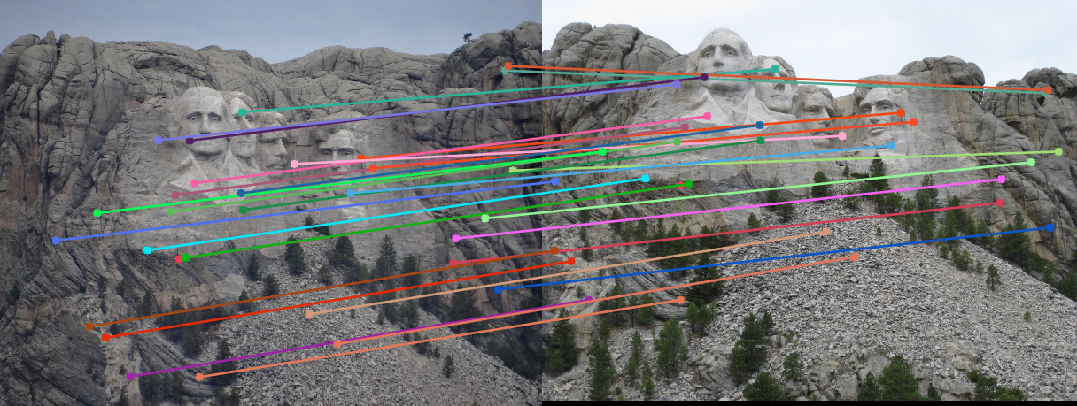
This section of the project is where we expand on the work that was done in the previous one. We're given lots of potential matches via the SIFT algorithm, but at the same time, we want to weed out outliers. So what do we do? We go through multiple iterations of checking the matches and checking that they hold up fine. For each iteration, we pick a random sample of 8 potential matches, and estimate the fundamental matrix based on those 8 samples. We then proceed to check each match against the estimated fundamental matrix and if the difference is within a certain threshold (say, +/- 0.05 because that's the classic number for statistical significance), we consider it to be an inlier and add it to our overall set of inliers. Once we've figured out the inliers, we can use the group of them to determine our best estimate of the overall fundamental matrix. Long story short, the process is check if a match works locally compared to a small subset of other matches and if it's good there, we assume it to be good overall. This works in general because for the most part the matches have the right idea and it's just a few spurious outliers in the mix, so it'd have to be pretty bad luck to randomly get a set of spurious matches that happen to be equally bad at representing the overall matches and skewed the same way. With that said, once we have our inliers, we also randomly select a subset of them to represent the inliers as a whole. It's entirely possible for some spurious points to become classified as inliers, so randomly selecting a subset of the inliers allows us to eliminate some of these as well. For the purposes of this project, I chose to pick 30 (makes the line visualizations nicer to look at and easier to verify). It wasn't necessarily needed for Mount Rushmore, as seen in the table below (first row is with all found inliers, second row is with 30 randomly selected inliers), but it was useful for some of the other images. The table below has images from left to right showing all the SIFT matches originally fed into the RANSAC algorithm, each image's epipolar lines generated from the fundamental matrix estimated from the inliers after RANSAC, and the inliers selected by RANSAC. Note that the epipolar lines end up converging in more or less the same area for both methods for the Mount Rushmore images, but this speaks to the quality of inliers that the SIFT algorithm was able to generate in this particular case and the general lack of very spurious outliers. However, the same cannot necessarily be said for other images as will be examined shortly.
|
|
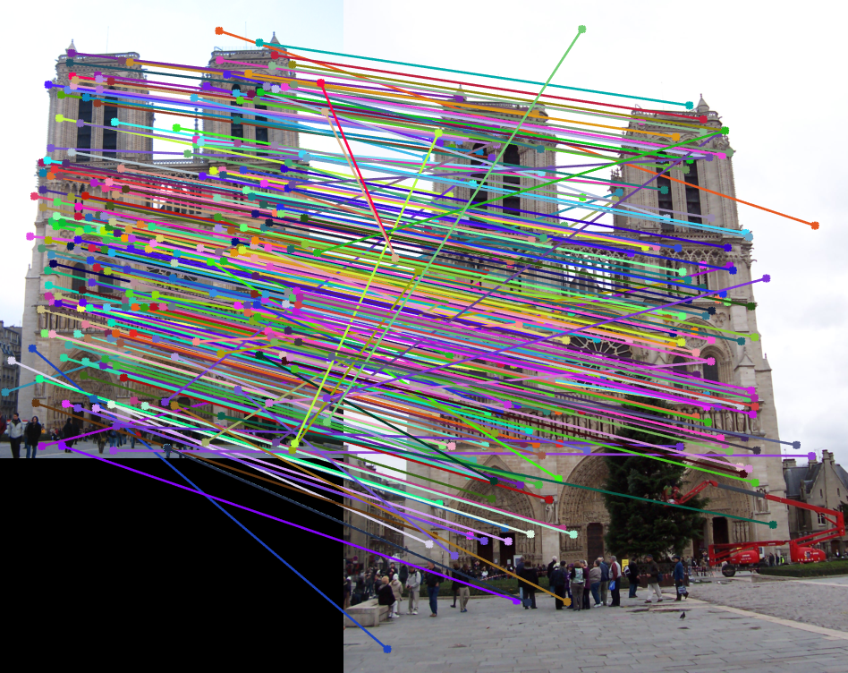
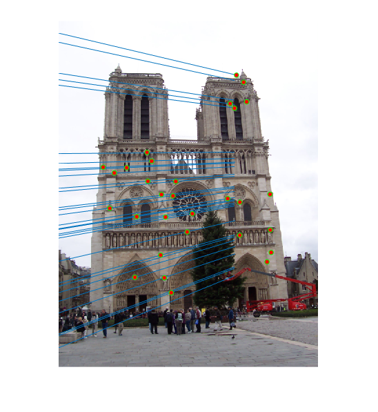
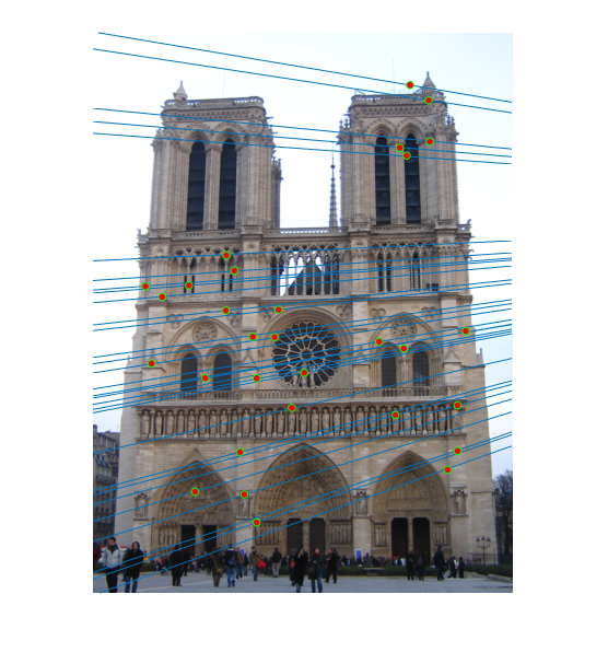
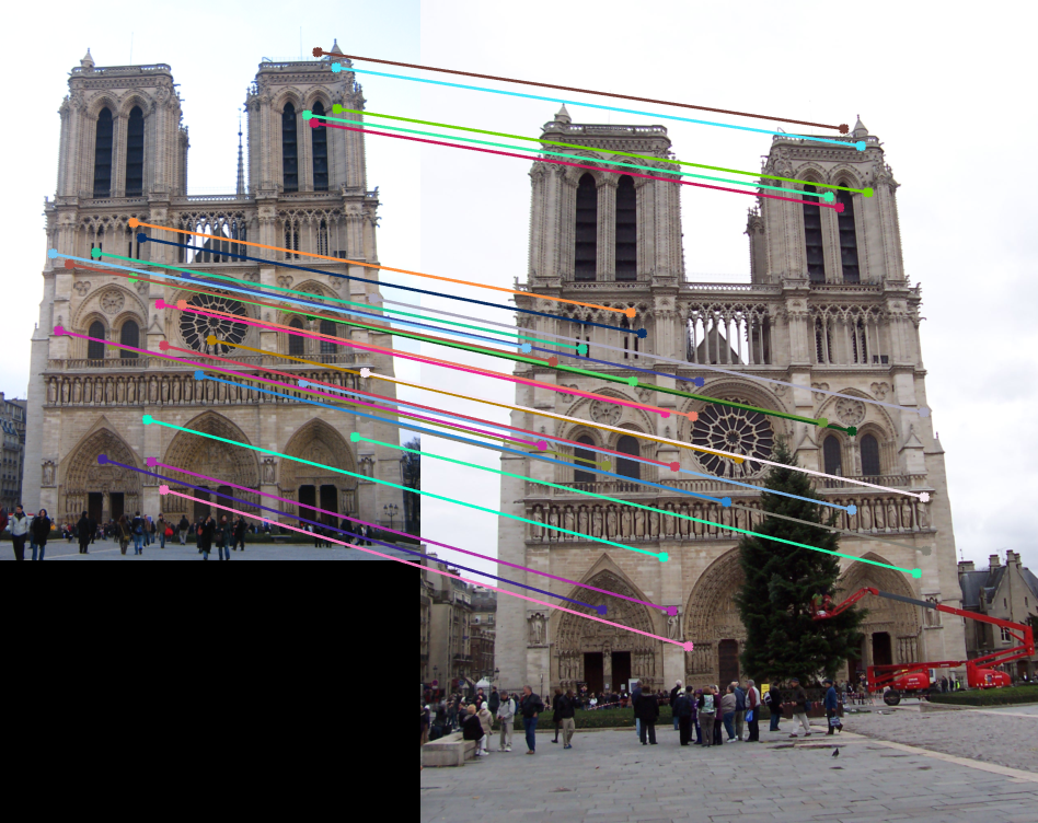
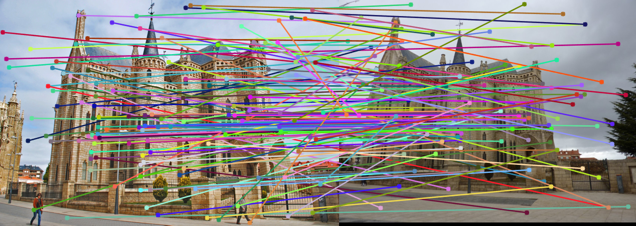
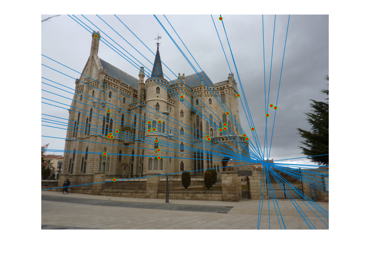
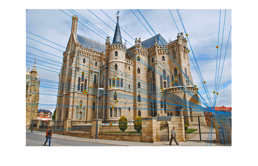
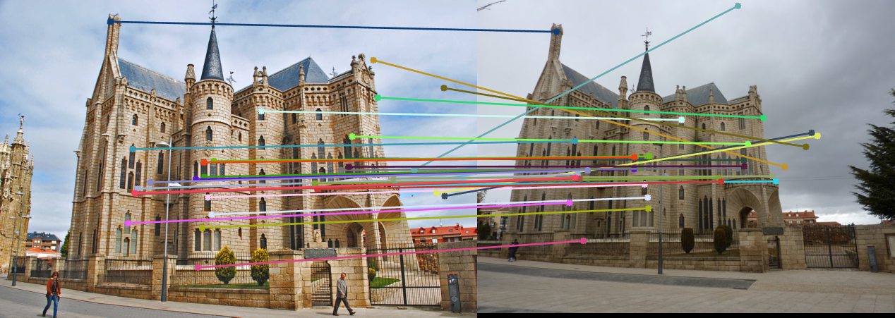
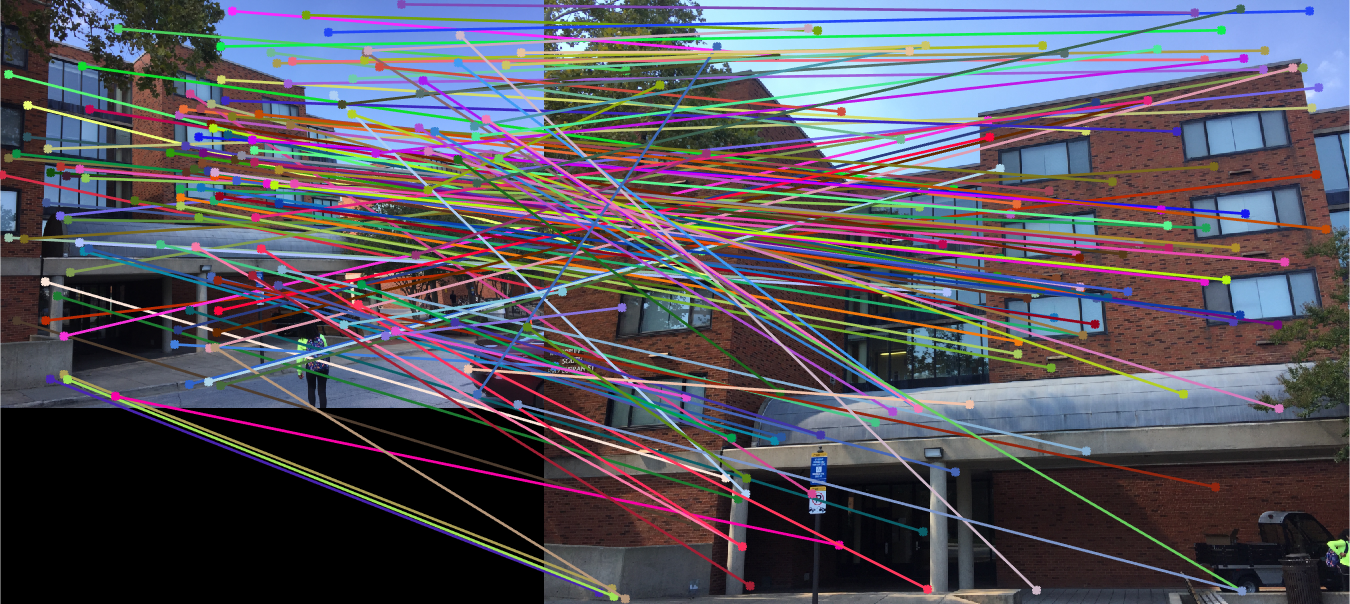
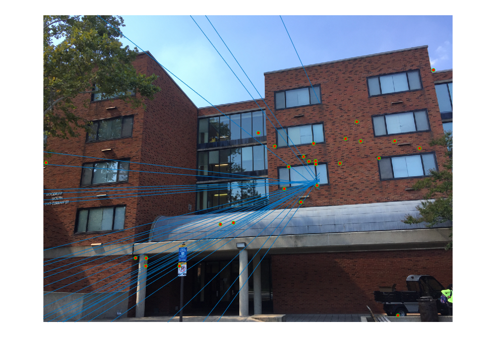
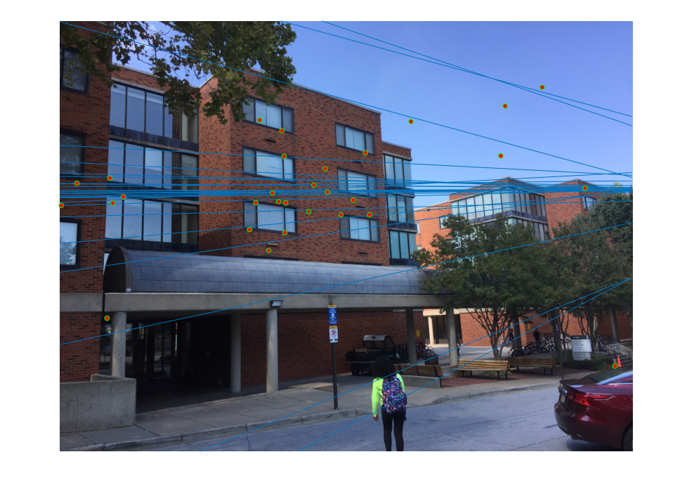
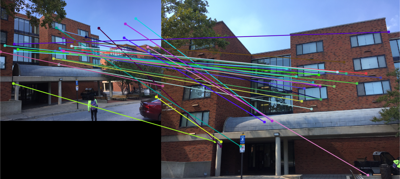
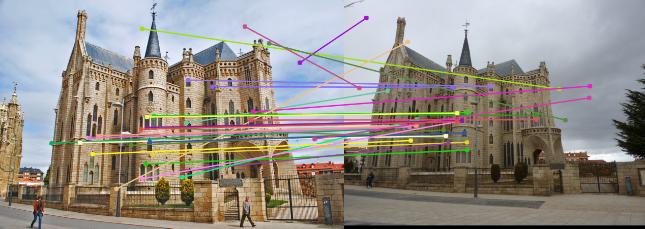
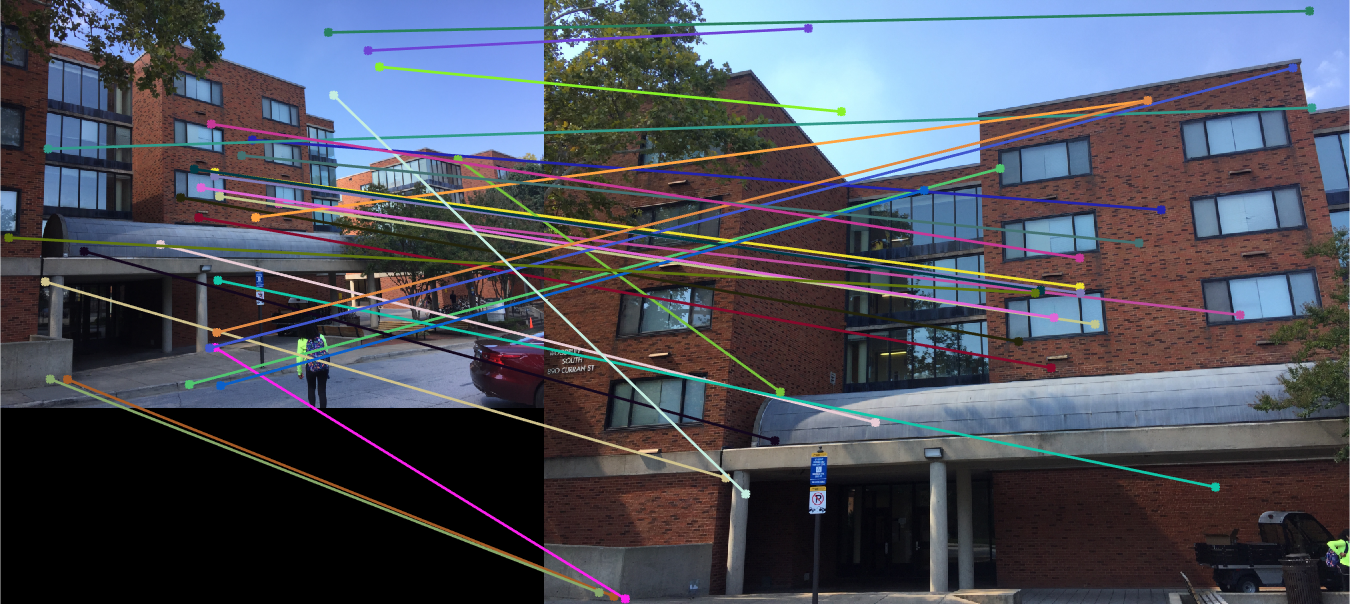
If you look below, you can see the results for some of the other images (presented in the same order of all SIFT matches, epipolar lines for image 1, epipolar lines for image 2, and exclusively inliers selected by RANSAC). As you can see, the results are not necessarily as perfect as with the Mount Rushmore set, but the implemented RANSAC algorithm does a fairly good job of picking inliers in general. From top to bottom, the rows correspond to using the Notre Dame images, the Episcopal Gaudi images, and the Woodruff images. The Episcopal Gaudi and Woodruff results were generated via fundamental matrix normalization, which will be explained next. Note that in particular, the algorithm was able to produce great results for the Episcopal Gaudi images, with only one or two insanely suprious matches being included and that for Woodruff the algorithm weeded out many of the outliers although some also found their way into the final result.
|
|
|
It's possible to improve the accuracy of the RANSAC algorithm via normalization of the fundamental matrix. More specifically, we're normalizing the coordinates in the calculation of the fundamental matrix, and then applying a similar transform on the matrix itself to convert it back to the original system it was dealing with. The scaling strategy that was used was for a particular set of coordinates, the minimum between the reciprocal of the standard deviation of the x values and the reciprocal of the standard deviation of the y values was used for the scaling factor. This is illustrated in the code snippet below.
  if normalize_f_matrix
      c_u = mean(Points_a(:, 1));
      s1 = 1/std(Points_a(:, 1) - c_u);
      c_v = mean(Points_a(:, 2));
      s2 = 1/std(Points_a(:, 2) - c_v);

      s_a = min([s1 s2]);

      Points_acheck = Points_a;
      Points_acheck(:, 3) = 1;
      transform_a = [s_a 0 0; 0 s_a 0; 0 0 1]*[1 0 -c_u; 0 1 -c_v; 0 0 1];
      T_a = [s_a 0 0; 0 s_a 0; 0 0 1]*[1 0 -c_u; 0 1 -c_v; 0 0 1]*Points_acheck';
      A_norm = T_a';
      A_norm(:,3) = [];
      Points_a = A_norm;

      c_u = mean(Points_b(:, 1));
      s1 = 1/std(Points_b(:, 1) - c_u);
      c_v = mean(Points_b(:, 2));
      s2 = 1/std(Points_b(:, 2) - c_v);

      s_b = min([s1 s2]);

      Points_bcheck = Points_b;
      Points_bcheck(:, 3) = 1;
      transform_b = [s_b 0 0; 0 s_b 0; 0 0 1]*[1 0 -c_u; 0 1 -c_v; 0 0 1];
      T_b = [s_b 0 0; 0 s_b 0; 0 0 1]*[1 0 -c_u; 0 1 -c_v; 0 0 1]*Points_bcheck';
      B_norm = T_b';
      B_norm(:, 3) = [];
      Points_b = B_norm;
  end
Note that we have variables T_a and T_b in the calculation of the normalized points, which are treated as the original points themselves for the calculation of the matrix. These represent the matrices that need to be multiplied with the fundamental matrix calculated via the normalized points so that we can convert the final matrix back to the original coordinate system being used. Normalizing the coordinates reduces the effect of outlier points that are randomly selected to estimate the fundamental matriix, and are thus less likely to be included when checking whether they are likely inliers. With the table below, consider the without normalization and with normalization results of inliers for Episcopal Gaudi and Woodruff. Note that some of the outliers tend to not be misclassified as inliers once we utilize this normalization method. In particular with Woodruff, there were multiple ridiculously spurious matches that were classified as inliers without doing the normalization. Doing the normalization for the most part helped in getting rid of some of them, although some remained. If anything, it mitigated the spurious matches to some extent.
|
|