Project 3 / Camera Calibration and Fundamental Matrix Estimation with RANSAC
The Algorithm
Part 1
Find the Camera Projection Matrix
In this part of the project, I created a matrix that would take 3D coordinates and compute their 2D coordinate counterparts.
-
Create a matrix representing a system of equations. Here, two rows of the matrix corresponds to row i of the 2D coordinate list and row i of the 3D coordinate list. Row i*2 - 1 uses the value of u and row i*2 uses the value of v. This creates a matrix with a height twice that of the initial lists. Using the points provided in each respective list, the following representation was created:
matrix(y,:) = [Xi Yi Zi 1 0 0 0 0 -ui*Xi -ui*Yi -ui*Zi ... 0 0 0 0 Xi Yi Zi 1 -vi*Xi -vi*Yi -vi*Zi]; -
Reorganize the matrix of u,v pairs such that it is one column resembling the following:
[u1 v1 u2 v2 ... un vn]; -
Next, divide the initial matrix containing the uv and XYZ relationships by the new, reorganized matrix of u,v pairs. This matrix could have many solutions, many of which are not helpful. For this reason, matrix(3,4) gets fixed to 1 during this step. Before this, the matrix contained 11 values, as the system of equations was represented. The 1 gets appended to the end, and the matrix gets reshaped to be a 3x4.
		M = matrix \ UV;
		M = [M; 1];
		M = reshape(M,[],3)';
Compute Camera Center
Here, the equation below is followed to retrieve the camera center:
		m4 = M(:, 4:4); % This takes a slice of matrix M equivalent to M's 4th (and last) column
		Q = M(:, 1:3); % This takes a slice of matrix M equivalent to M's first 3 columns
		Center = (-1 * inv(Q)) * m4;
Part 2
Fundamental Matrix Estimation
This part of the project is similar in form to the first, as it is simply mapping out a system of equations to then solve. This time, however, the matrix to be solved for is mapping one set of points to another set of points in the same plane. These points are homogenous.
-
Create the system of equations matrix. Each row will look like the row below:
u_prime = Points_a(y,1); v_prime = Points_a(y,2); u = Points_b(y,1); v = Points_b(y,2); matrix(:, y) = [u*u_prime u*v_prime u v*u_prime v*v_prime v u_prime v_prime 1]; - Here, we are using singular value decomposition to solve for our fundamental matrix from the system of equations we've set up!
[U, S, V] = svd(matrix); f = V(:, end); F = reshape(f, [3 3])'; - Here, we are reducing the rank of F, and finally, calculating for the final F.
			[U, S, V] = svd(F);
			S(3,3) = 0;
			F = U*S*V';
Part 3
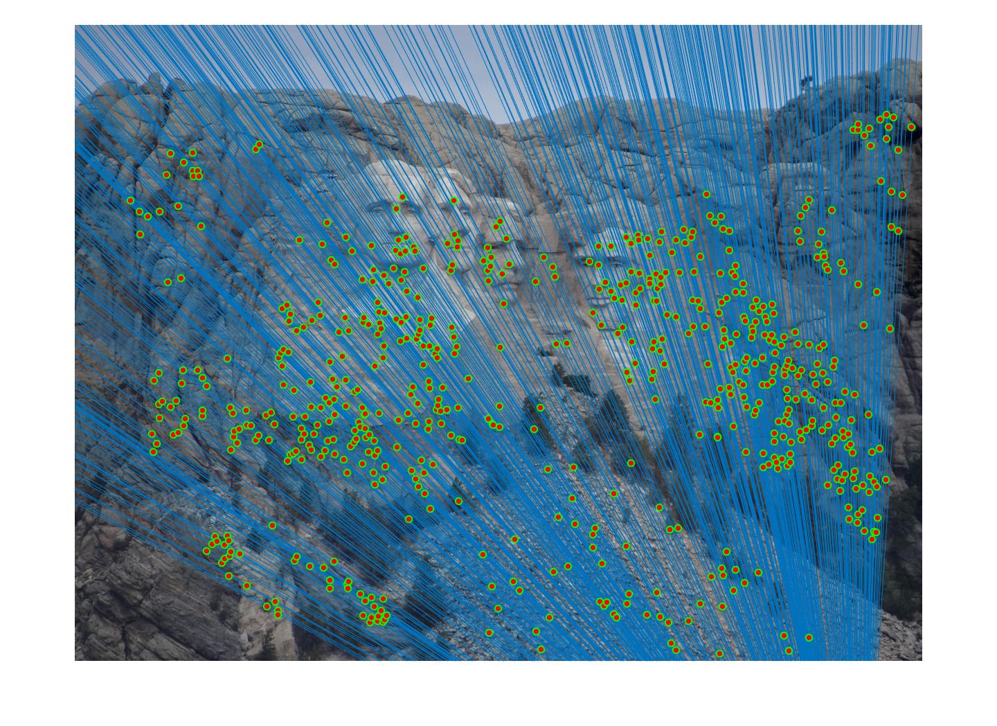
Find Fundamental Matrix with RANSAC
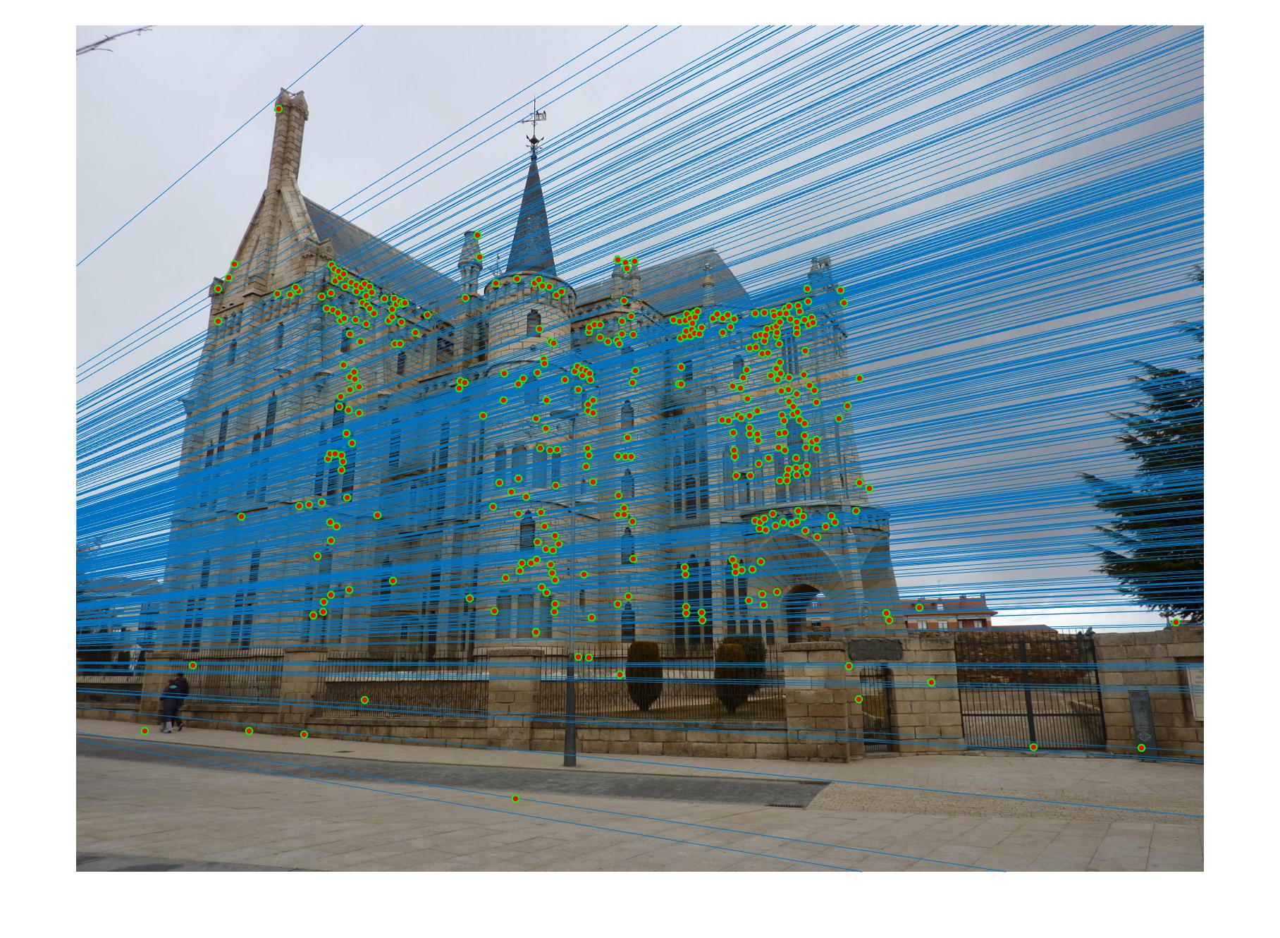
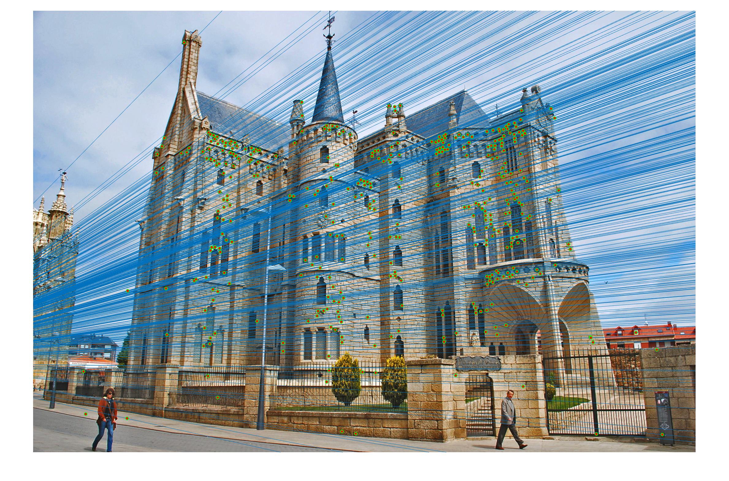
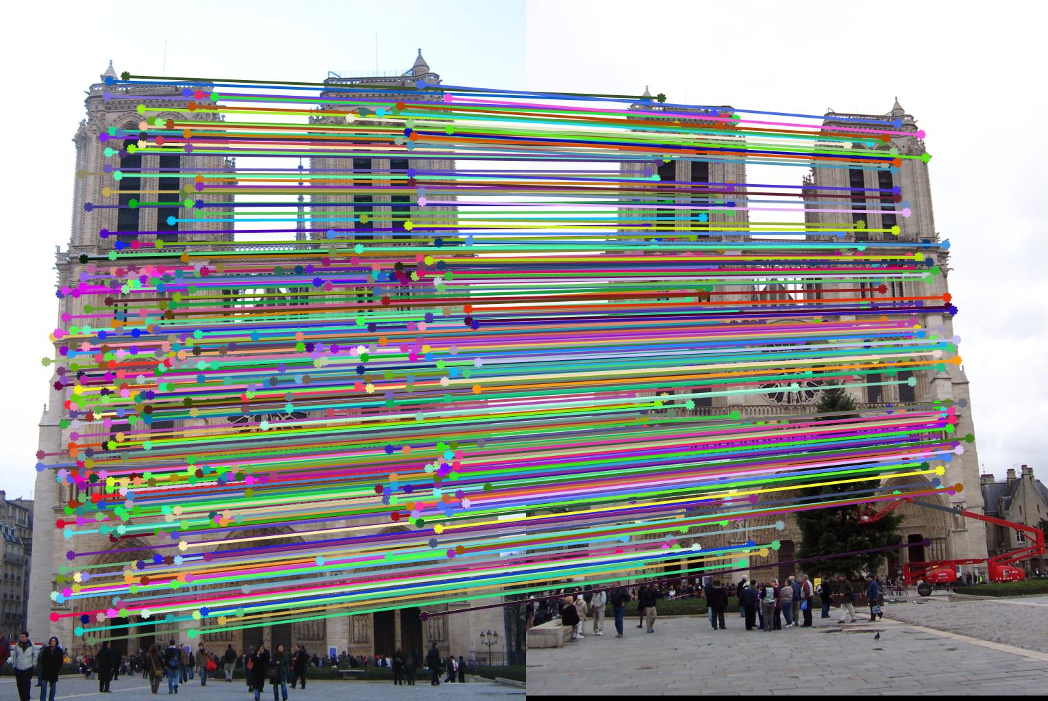
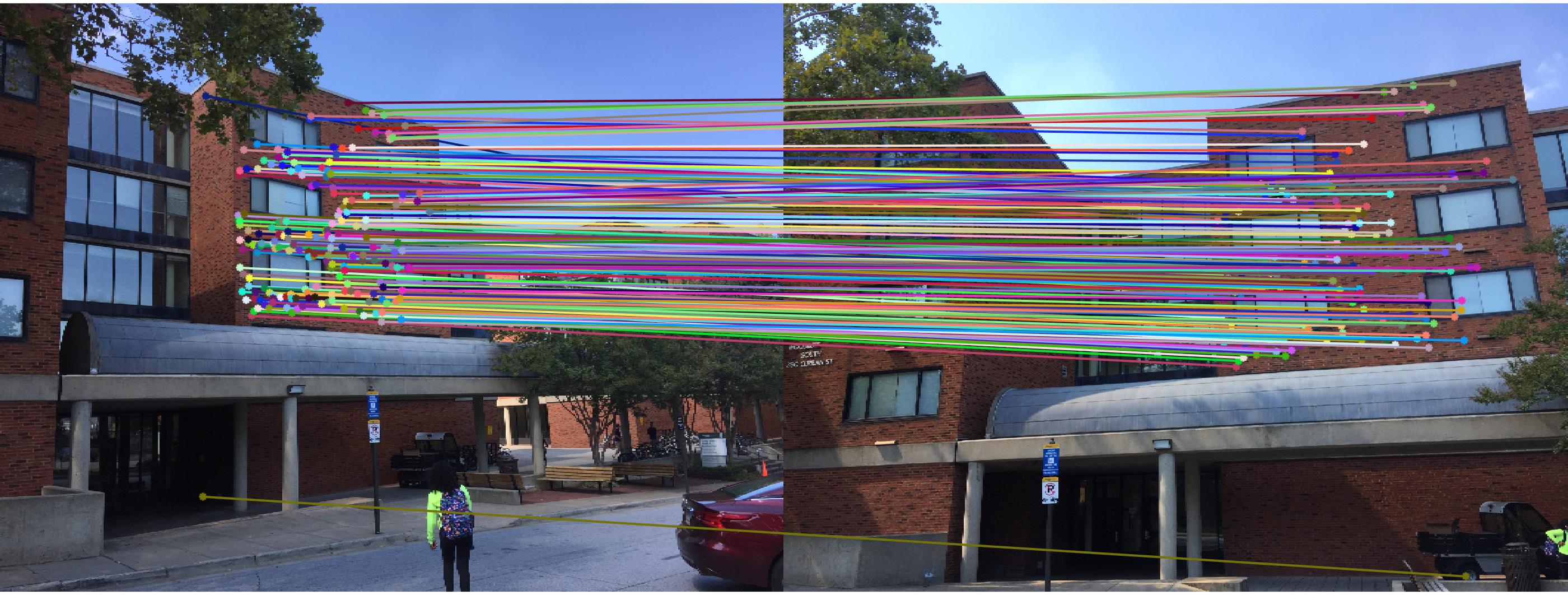
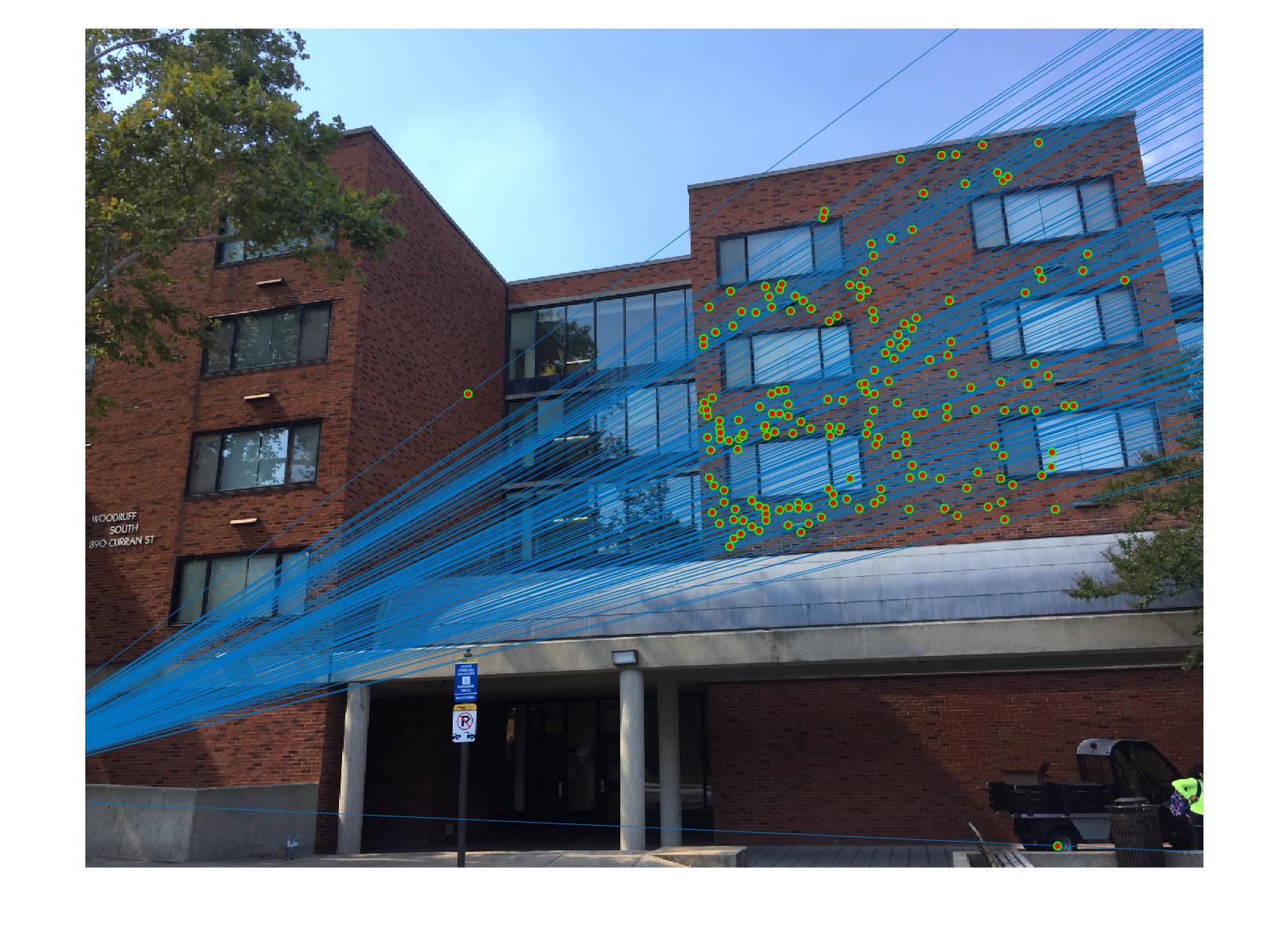
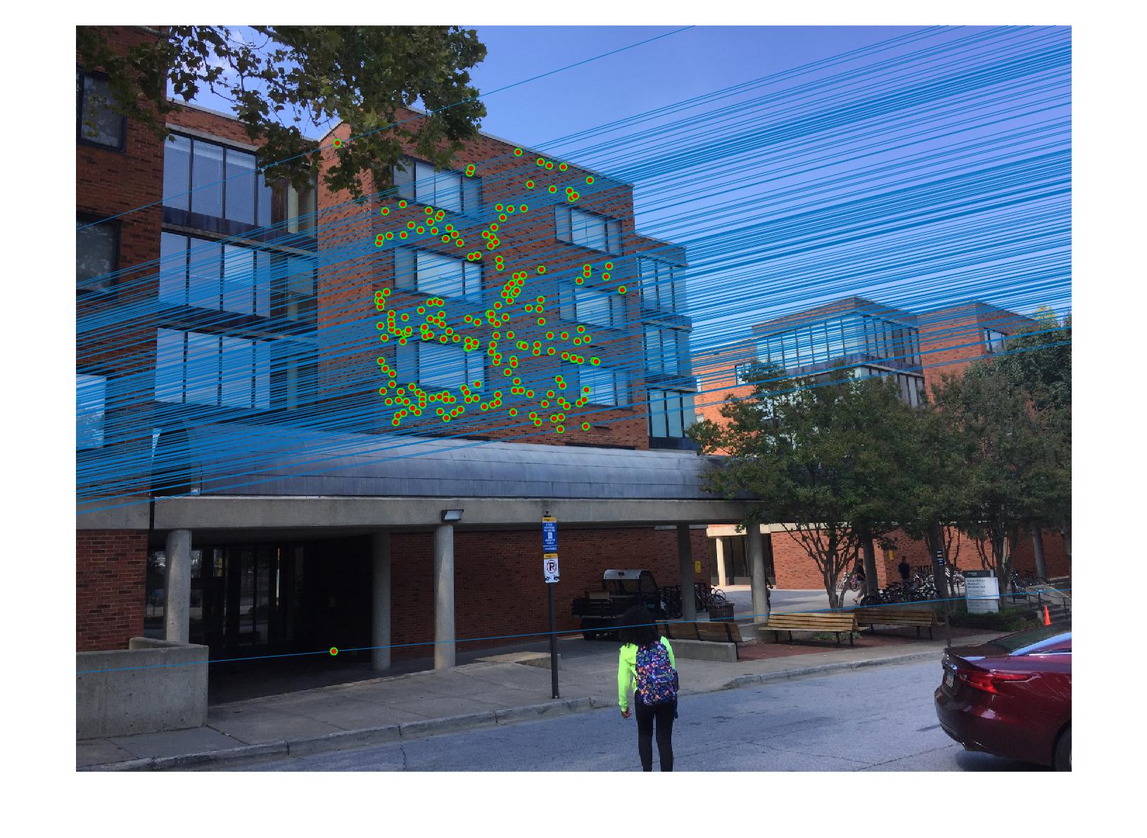
In this section, estimate_fundamental_matrix will get called repeatedly, as the algorithm searches for the "best" predictor. I decided to perform 1000 iterations, computing inliers for each fundamental matrix as I go. I have defined an outlier as any pair of values for which xFx' is not between -0.005 and 0.005. After computing inliers, I use the number of inliers to choose whether or not to replace the current "best fundamental matrix." After 1000 iterations, the best fundamental matrix (that which has the maximum number of inliers) and its inliers get returned. The range of -.005 to .005 was decided upon after testing many other options. This number is small enough so that it is selective, but not too conservative such that a small number of inliers gets returned.
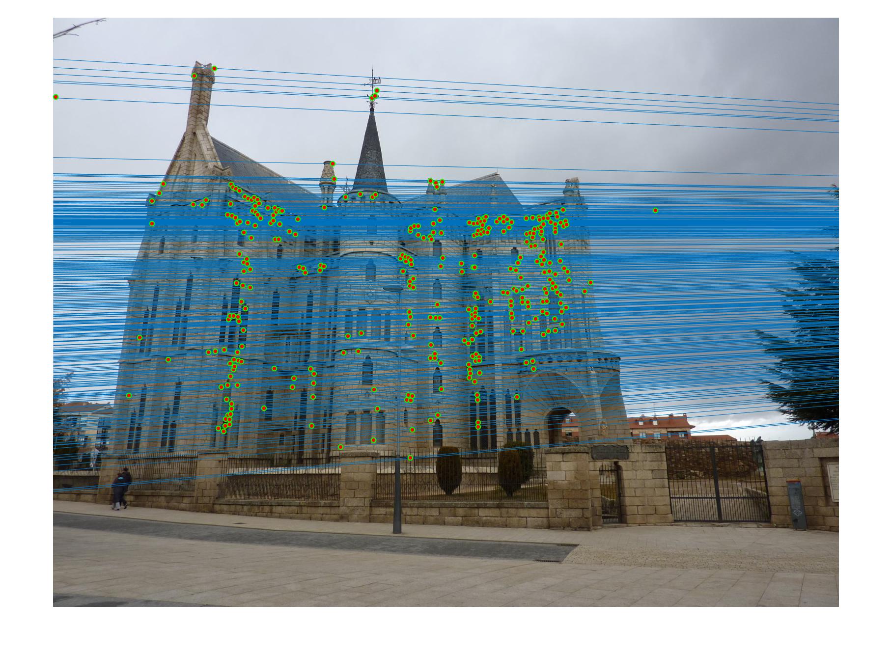
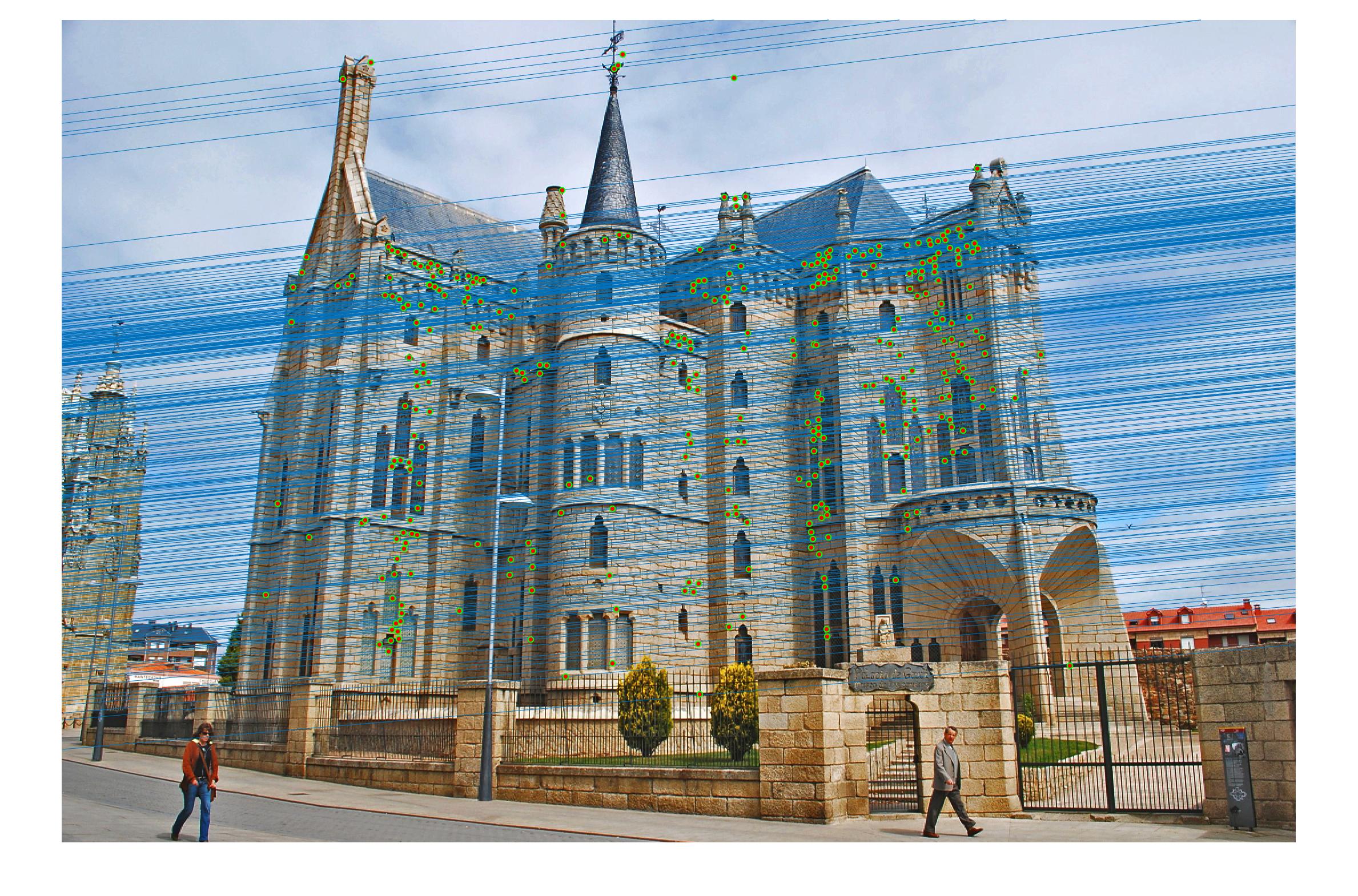
Extra Credit: Coordinate Normalization
Rescaling the data leads to better numerical conditioning. With much smaller discrepancies between numbers, the estimation becomes more precise with fewer rounding errors. This is performed as follows:
- Calculate the mean for u and v for each set of points. Subtract this mean from each set, respectively.
- Calculate the standard deviation of each set of points. Use this to create a scale value. Here, I used 1 / std deviation. Using this as a scale later will ensure that all points are within 1 standard deviation of each other.
- Multiply each set of points by its calculated scale value.
- Create a transformation matrix from scale and shift matrices for each set of points. See below:
- Transform the fundamental matrix away from the scaled and transformed points.
				a_scale_matrix = [a_scale,0,0;  0,a_scale,0;    0,0,1];
				a_shift_matrix = [1,0,-1*a_u_mean;  0,1,-1*a_v_mean;    0,0,1];
				a_transform = a_scale_matrix * a_shift_matrix;
F_matrix = b_transform' * F * a_transform;
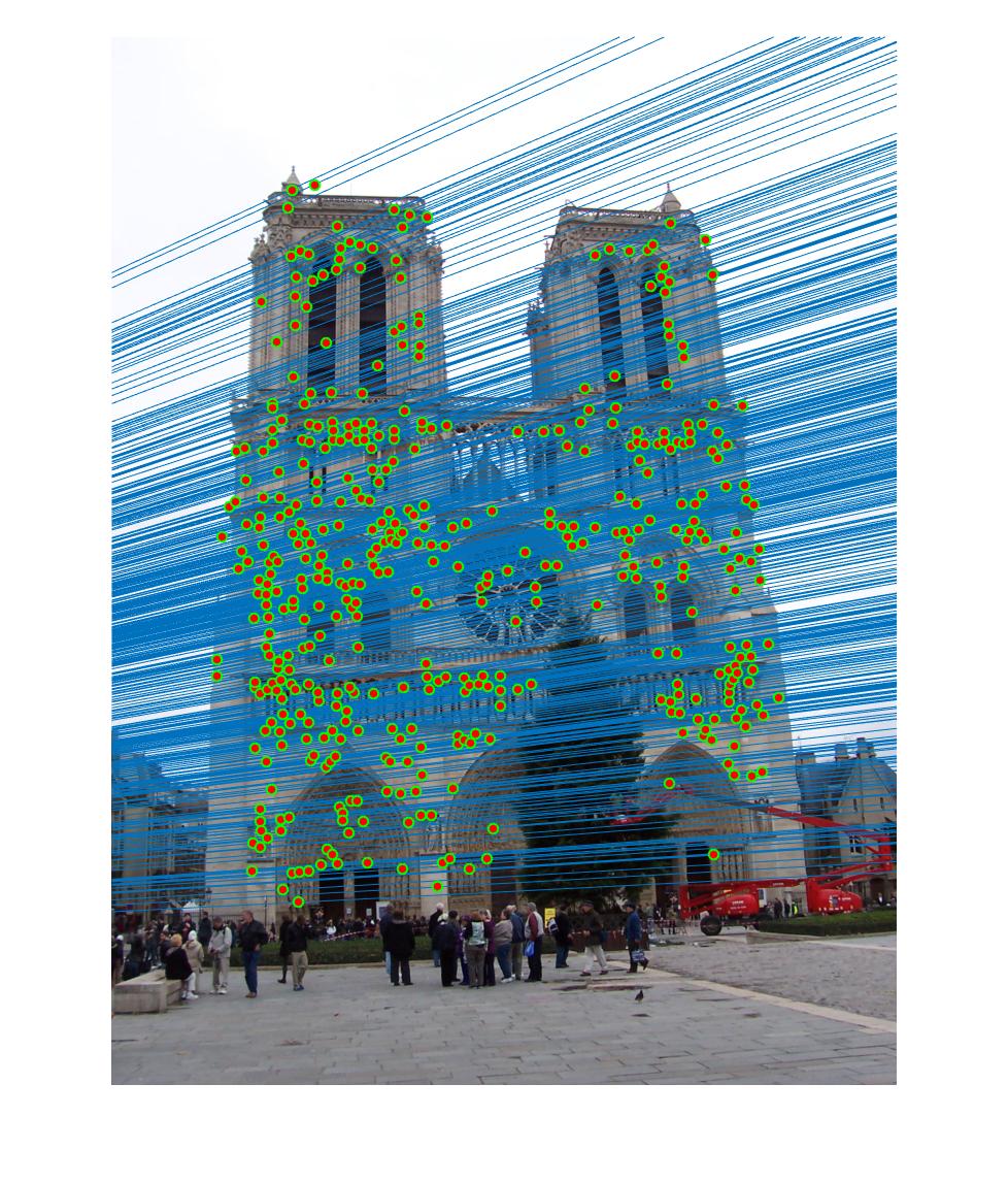
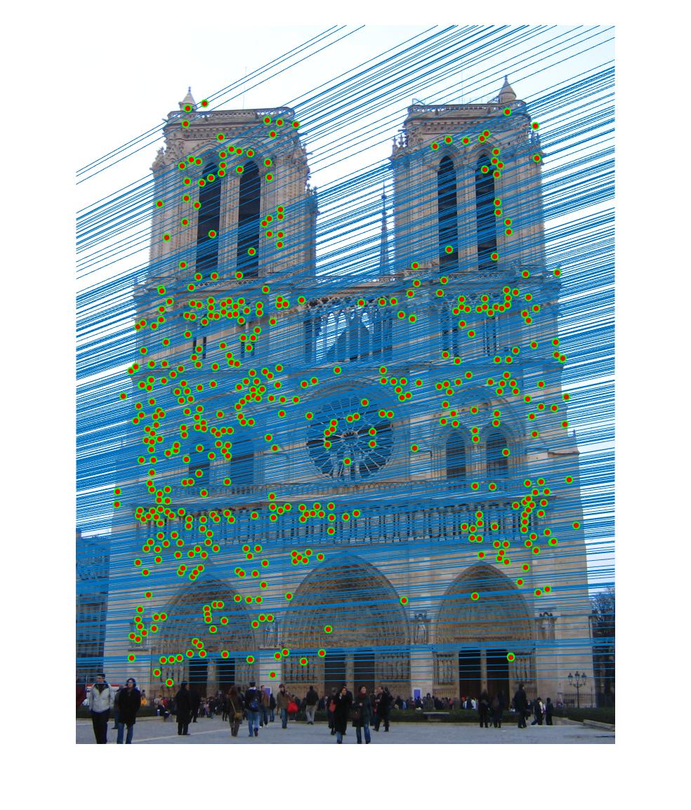
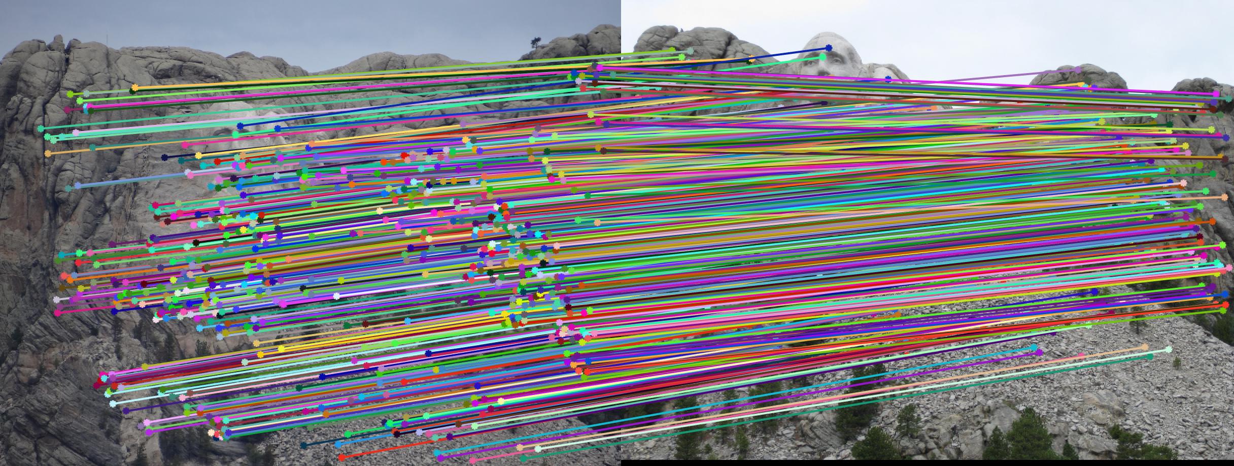
The effects:
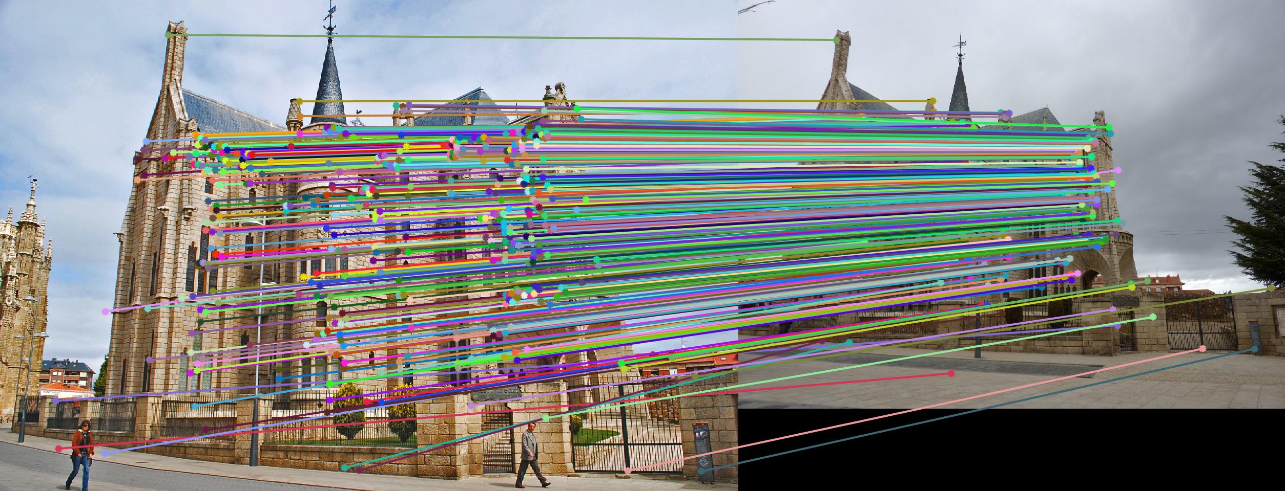 Before
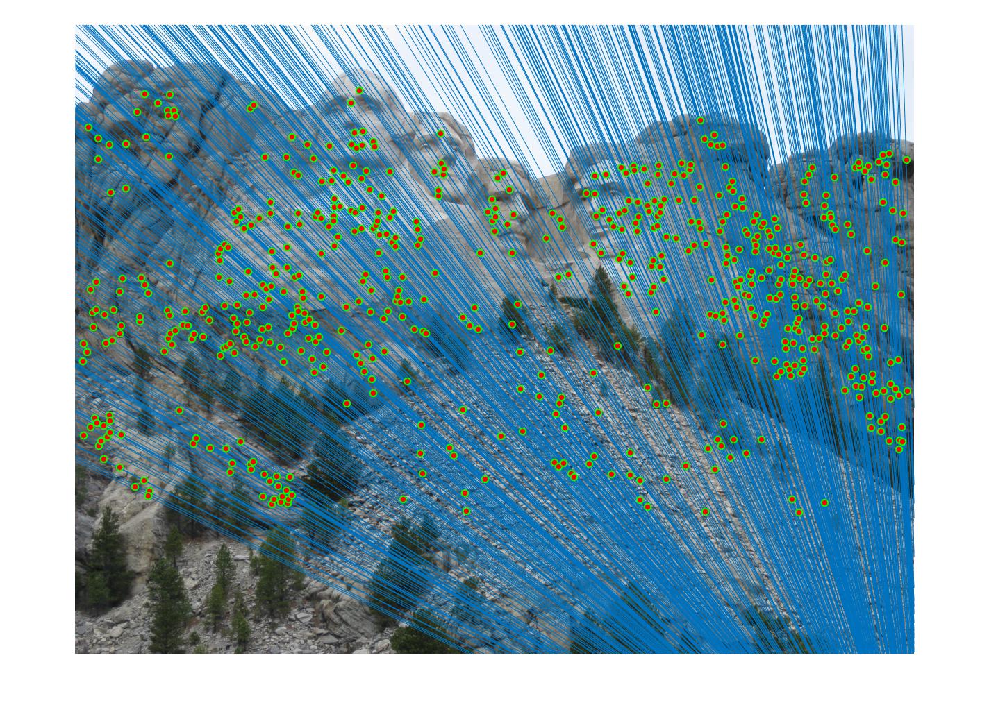
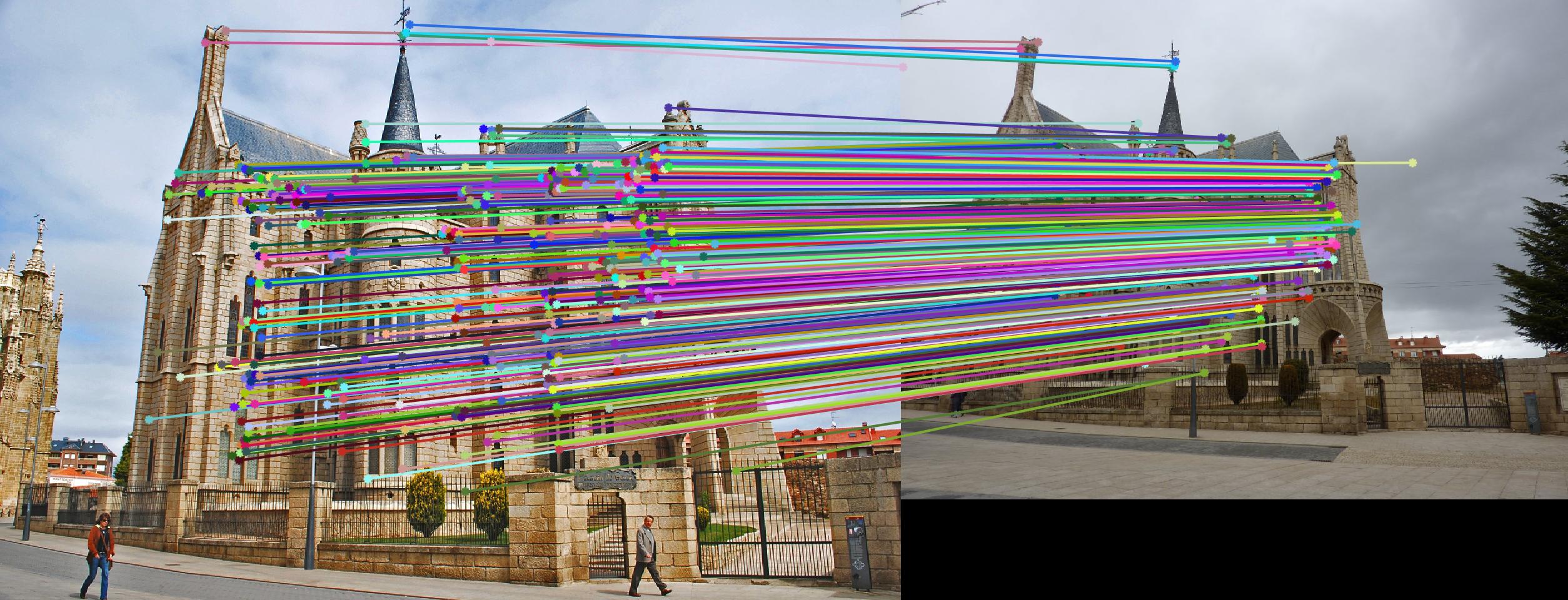 After
After