Amritha Ram

1. Estimating the Camera Projection Matrix

The camera projection matrix is the one that converts world 3D coordinates to 2D image coordinates. Using the equations provided in the project brief, specifically the following:

I was then able to solve for matrix M using Singular Value Decomposition. The matrix I found corresponded with the provided matrix M in the brief.

The projection matrix is:
0.4583 -0.2947 -0.0140 0.0040
-0.0509 -0.0546 -0.5411 -0.0524
0.1090 0.1783 -0.0443 0.5968

The residual was around 0.445.

Using this matrix and the information from lecture on how to find the camera center C, I used the inverse of the 3x3 within M, multiplied by the fourth column of M. This yielded the camera center correctly. The estimated location of camera was: <-1.5127, -2.3517, 0.2826>

Code snippet to create linear regression to find the elements of M:

E = zeros(2*numPoints, 12); %11 for the entries of the big matrix and 1 for the column of u or v.
for i = 1:numPoints
    point2d = Points_2D(i,:);
    point3d = Points_3D(i,:);
    u = point2d(1,1);
    v = point2d(1,2);
    x = point3d(1,1);
    y = point3d(1,2);
    z = point3d(1,3);
    row1 = [point3d 1 0 0 0 0 -u*x -u*y -u*z -u];
    row2 = [0 0 0 0 point3d 1 -v*x -v*y -v*z -v];
    E(2*i-1,:) = row1;
    E(2*i,:) = row2;
end

[U,S,V] = svd(E);
M = reshape(V(:,end), 4,3)';

2: Fundamental Matrix Estimation

The fundamental matrix is the one that helps us map points in one image to lines in another. Using a similar set up as from part 1 for the linear regression, we solve for F using SVD once again, estimate a rank 2 matrix by simply setting the lowest singular value to 0 and then performing SVD again.

The epipolar lines drawn on the sample images:

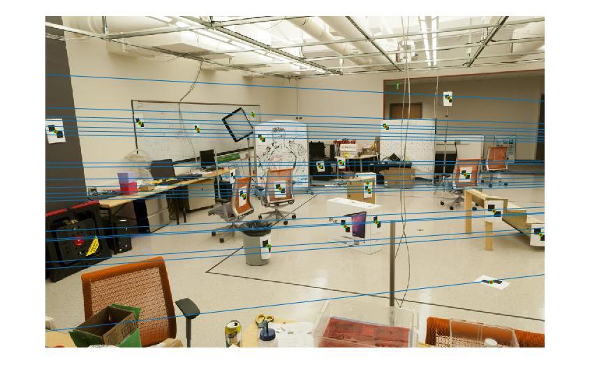
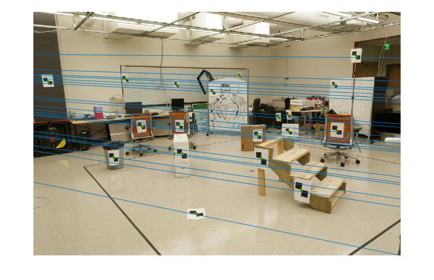
From glancing at the visualization and comparing with the provided lines, this points to correctness of our estimation of the fundamental matrix.

Fundamental matrix estimated =
-0.0000 0.0000 -0.0019
0.0000 0.0000 0.0172
-0.0009 -0.0264 0.9995

Code snippet to create linear regression to find the elements of M:

for i=1:numPoints
    a = Points_a(i, :);
    b = Points_b(i,:);
    ua = a(1,1);
    ub = b(1,1);
    va = a(1,2);
    vb = b(1,2);
    E(i,:) = [ua*ub va*ub ub ua*vb va*vb vb ua va 1];
end

[U,S,V]=svd(E);

F_matrix = V(:,end);
F_matrix = reshape(F_matrix, [3 3])';
% values arranged in descending order in S
[U,S,V] = svd(F_matrix);
S(3,3) = 0;

F_matrix = U * S * V';

Fundamental Matrix with RANSAC

For this section, we use RANSAC in conjunction with the original fundamental matrix estimation in order to best deal with the presence of multiple outliers. The starter code allows for us to use vl_sift to perform SIFT matching for the given image pairs, and use these point correspondences with RANSAC to find the most appropriate fundamental matrix. The basic steps were as follows:

• Iteratively choose 8 number of point correspondences from the given list.
• Solve for the fundamental matrix using these correspondences.
• Count the number of inliers, i.e point correspondences that lie within a certain threshold of the model set up by our estimated fundamental matrix. Using the property of the fundamental matrix that for a correspondence (x1,x2), x2*F*x1' = 0, we pick a threshold such that lower values suggest higher agreement with the model. The threshold I chose to use was 0.006 after multiple tries and a general estimation of results from visualizations.
• Repeat this process some number of times (my implementation used 3000 iterations)

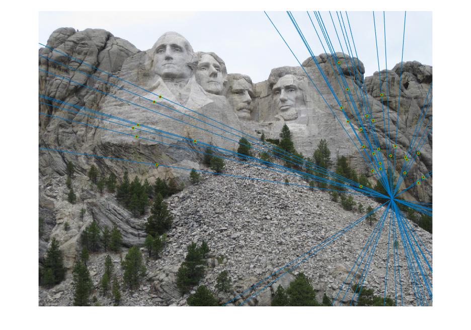
Results:

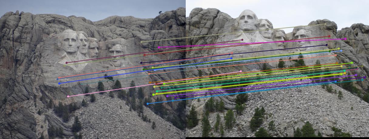
Mount Rushmore Image pair:

Epipolar lines on images: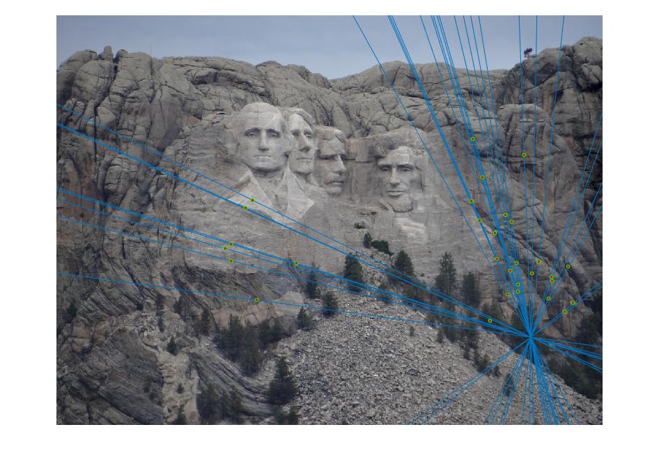

Visualization of matches:

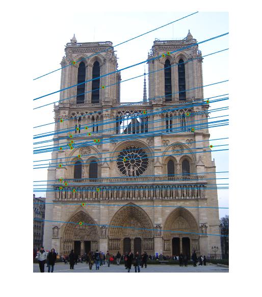
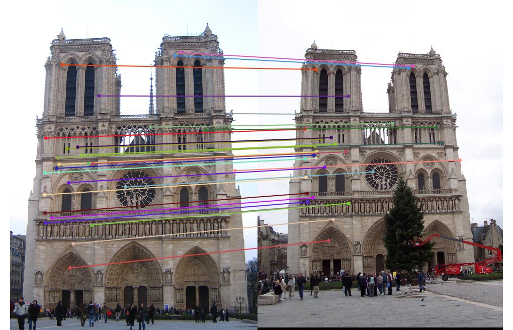
Notre Dame Image pair:

Epipolar lines on images: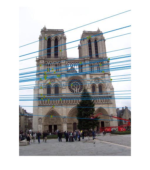

Visualization of matches:

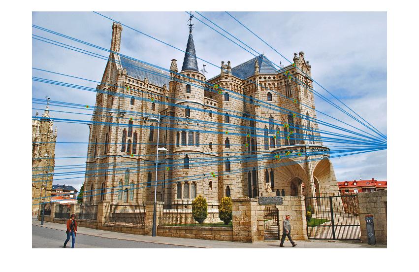
Episcopal Gaudi Image pair:

Epipolar lines on images: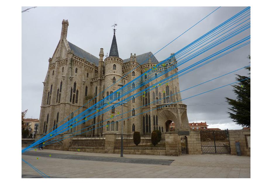

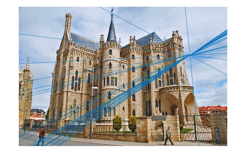
Visualization of matches:


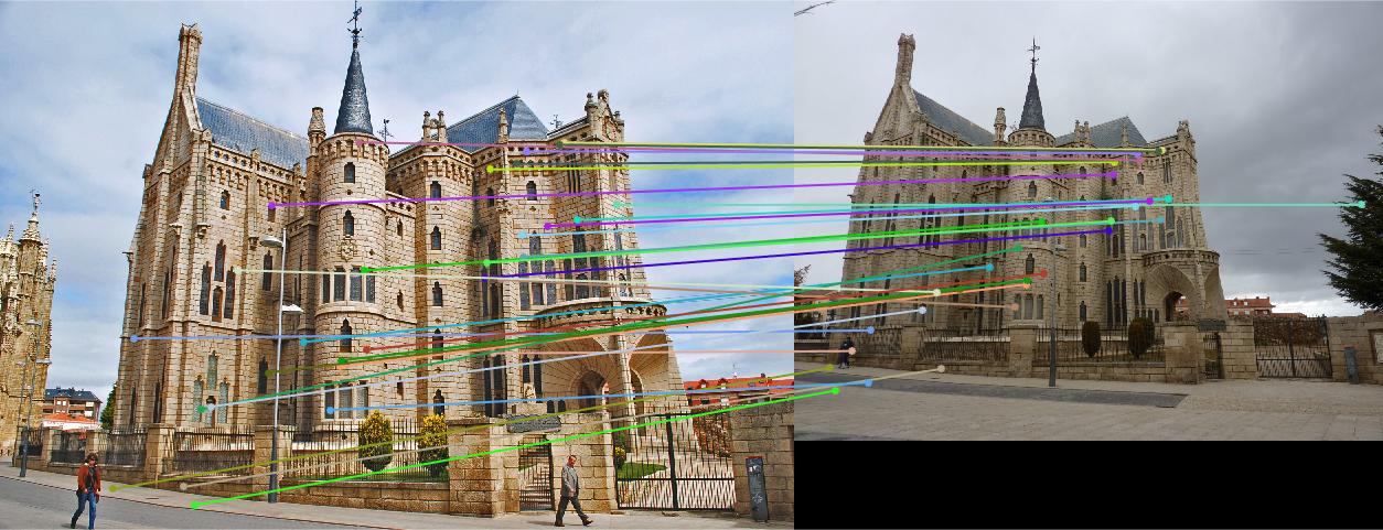
In the above cases, I randomly chose 30 of the inliers of the fundamental matrix model to represent for a cleaner visualization, which is still quite indicative of how the matches perform overall. Episcopal Gaudi still provided quite a few spurious matches and there are still issues with the fundamental matrix calculation not being well constrained, but the results shown above do indicate good accuracy in general or fewer outliers.

Extra credit portion: Normalization

After obtaining the above results, I implemented coordinate normalization prior to fundamental matrix estimation. For this, I computed the means and chose to scale the coordinates on the computation of their standard deviations (see following code snippet), and then adjusted the fundamental matrix as well as per the equation given in the brief where F_orig = T_b' * F_normalized * T_a.

Code snippet to normalize points and compute transformation matrices:

numPoints = size(Points_a, 1);
sum_a = sum(Points_a);
cu_a = sum_a(1,1)/numPoints;
cv_a = sum_a(1,2)/numPoints;
sum_b = sum(Points_b);
cu_b = sum_b(1,1)/numPoints;
cv_b = sum_b(1,2)/numPoints;

Us_a = Points_a(:, 1) - cu_a;
Vs_a = Points_a(:, 2) - cv_a;
scale_a = sqrt(sum(Us_a.^2 + Vs_a.^2));

Us_b = Points_b(:,1) - cu_b;
Vs_b = Points_b(:,2) - cv_b;
scale_b = sqrt(sum(Us_b.^2 + Vs_b.^2));

T_a = [scale_a, 0,0; 0, scale_a, 0; 0, 0, 1];
T_a = T_a * [1, 0, -cu_a; 0, 1, -cv_a; 0,0,1];
T_b = [scale_b, 0,0; 0,scale_b,0; 0,0,1];
T_b = T_b * [1,0,-cu_b; 0,1,-cv_b;0,0,1];

The results on the Episcopal Gaudi Image pair were as follows:

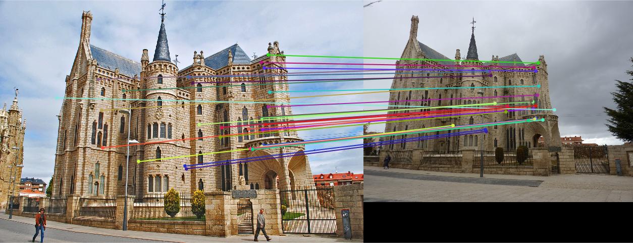
Visualization of matches:

Epipolar lines:

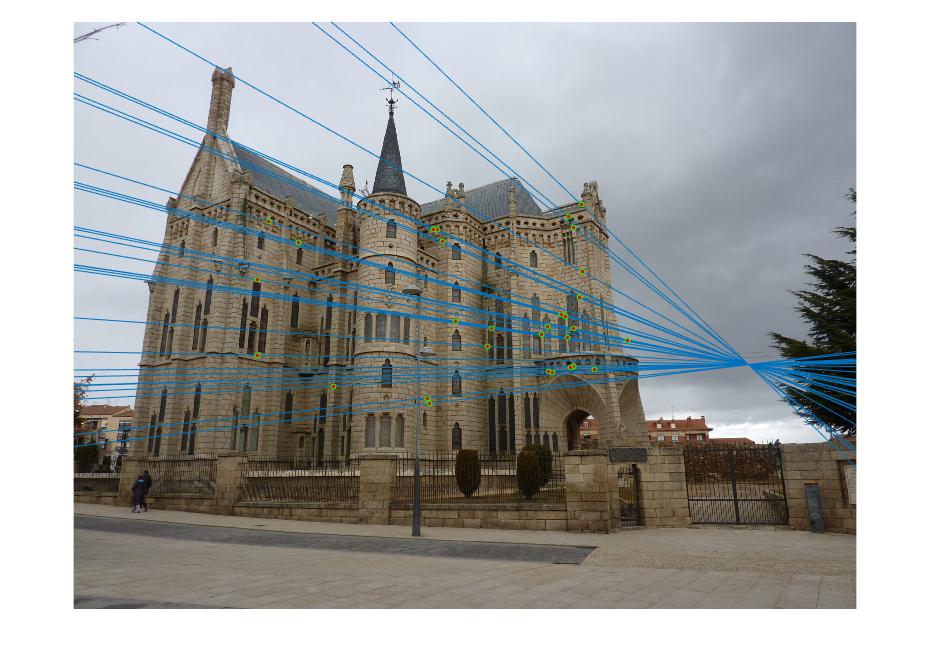
The matches for the other pairs of images were already quite good, but comparing to the pre-normalized points from before, Episcopal Gaudi seemed to perform much better after normalization. There do seem to be 1 or 2 spurious matches, but the overall improvement is evident.