Project 3 / Camera Calibration and Fundamental Matrix Estimation with RANSAC
The project consists of three parts:
- Estimating the projection matrix
- Estimating the fundamental matrix
- Estimating the fundamental matrix with unreliable SIFT matches using RANSAC
Part I: Camera Projection Matrix
Here, we estimate the camera projection matrix, which maps 3D world coordinates to image coordinates.
Using homogeneous coordinates, the equation for moving from 3D world to 2D camera coordinates is:

We write this equation in the form Am = 0, and solve for 'm' using linear least squares.

M gives the camera projection matrix. Once we have the projection matrix, it is easy to find the matrix K and the matric [R|T] of extrinsic parameters, such as the camera center in world coordinates.
We know that M = (Q|m4)
The center of the camera can be found by simply computing C = -Q-1m4
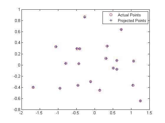
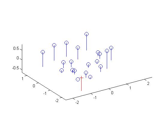
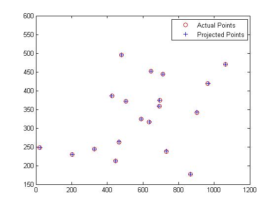
The following results are obtained for the given normalized 3D coordinates:

The figures below show the estimated 3D location of the camera with respect to the normalized 3d point coordinates:
Now, computing the projection matrix and camera centers for the given 3D points without normalization:

The figures below show the estimated 3D location of the camera with respect to the normalized 3d point coordinates:
Part II: Fundamental Matrix Estimation
Here, we map points in one image to lines in another by means of the fundamental matrix. We know that the fundamenta matrix is given by:


Part II: Extra Credit - Normalizing coordinates
Estimation of the fundamental matrix can be improved by normalizing the coordinates before computing the fundamental matrix. The method mentioned above is standard, but if applied naively it's quite unstable. In real world images, the source and target coordinates are usually noisy, and could have large variance. A simple solution would be to normalize the image coordinates before estimating the fundamental matrix. This provides a very well balanced matrix A (if using the least squares estimate) and a much more stable and accurate results for the fundamental matrix F.
%Function to normalize coordinates:
function [X, T ] = normalize(x)

n = size(x,1);

C = mean(x);
%Subtract means
x_new(:,1) = x(:,1) - C(1);
x_new(:,2) = x(:,2) - C(2);

%Compute standard deviation for mean shifted data
s_u = 1/std(x_new(:,1));
s_v = 1/std(x_new(:,2));

%Transformation matrix
%T = scale matrix x offset matrix
T = [s_u 0 0; 0 s_v 0; 0 0 1] * [1 0 -C(1); 0 1 -C(2); 0 0 1];

% Normalized coordinates
X = (T * [x ones(n,1)]')';
end

...

% Compute Fundamental matrix
F_matrix = T2' * F_norm * T1;
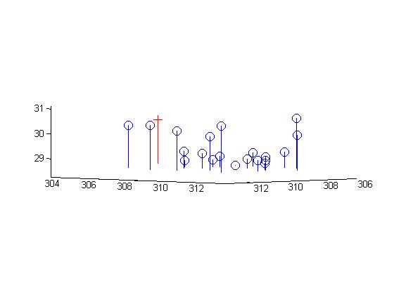
We test the fundamental matrix estimate by drawing the epipolar lines on one image which correspond toa point in the other image. The fundamental matrix is found to be:
Fmatrix =

Part III: Fundamental Matrix with RANSAC
Here, point correspondences for 2 photographs of a scene are computed using SIFT.However, these point correspondences are very unreliable. Therefore, to compute the fundamental matrix from this noisy data, we use RANSAC in conjunction with the fundamental matrix estimation to filter away spurious matches and achieve near perfect point correspondence.
The algorithm used is given below:

Values used:
p = 0.99
threshold = 0.05
Maximum no. of Trials = 4000
Results
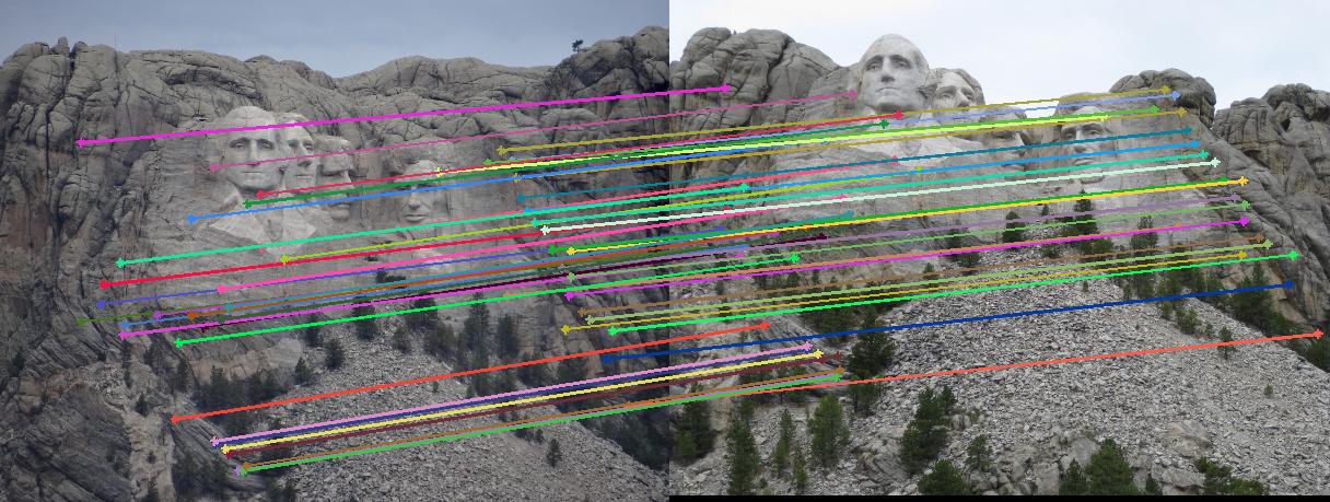
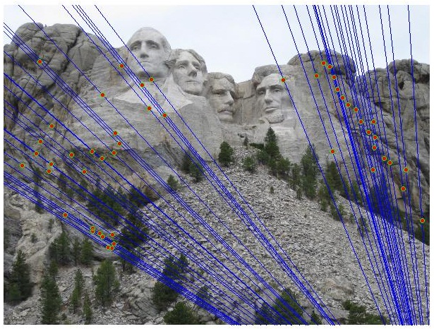
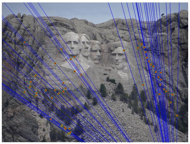
Mount Rushmore
Inlier Keypoint correspondence:
Epipolar lines:
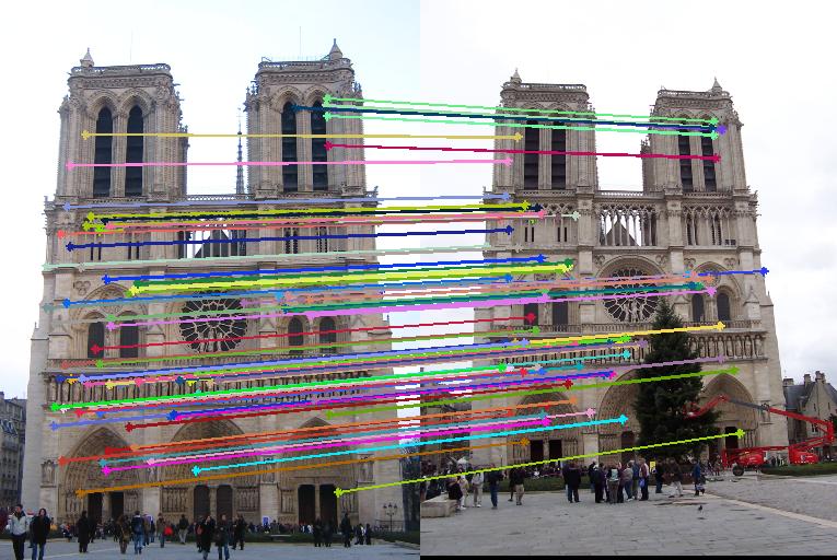
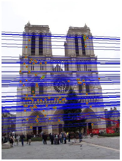
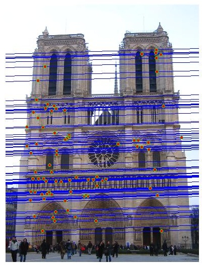
Notre Dame
Inlier Keypoint correspondence:
Epipolar lines:
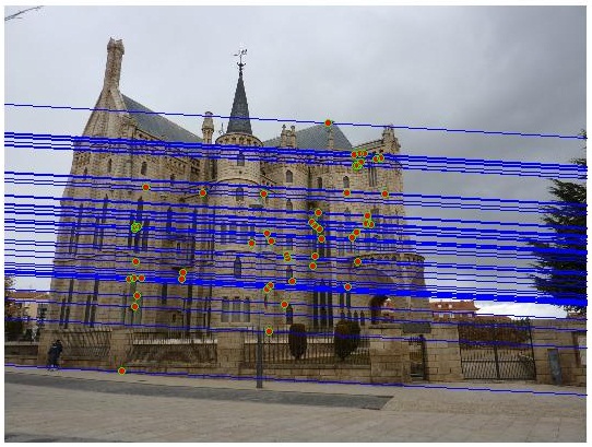
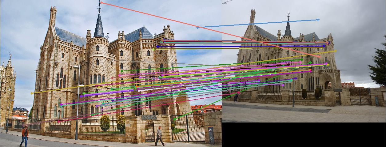
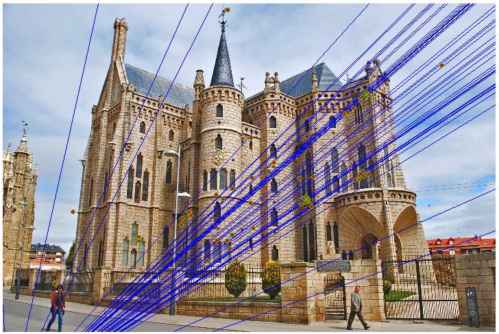
Episcopal Gaudi
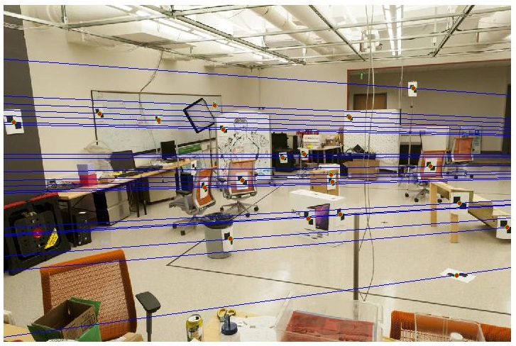
The episcopal Gaudi image pair doesn't produce many correct matches unless the comparision is performed at high resolution. This would result in tens of thousands of SIFT features, and time to process these features would be large. We see here that the keypoint correspondences found are very poor (they consist of largely spurious matches).
Inlier Keypoint correspondence:
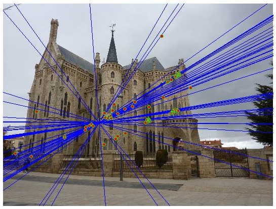
Epipolar lines:
As is seen from epipolar lines in the figures below, the fundamental matrix estimated is not very reasonable.
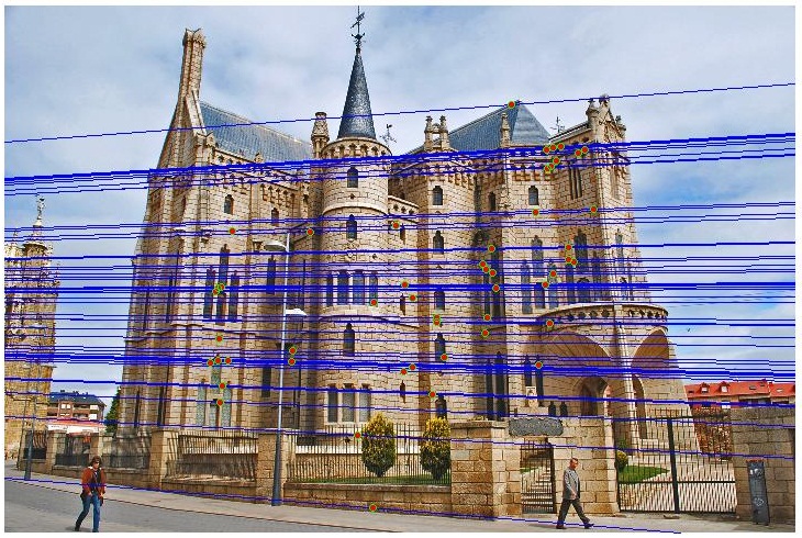
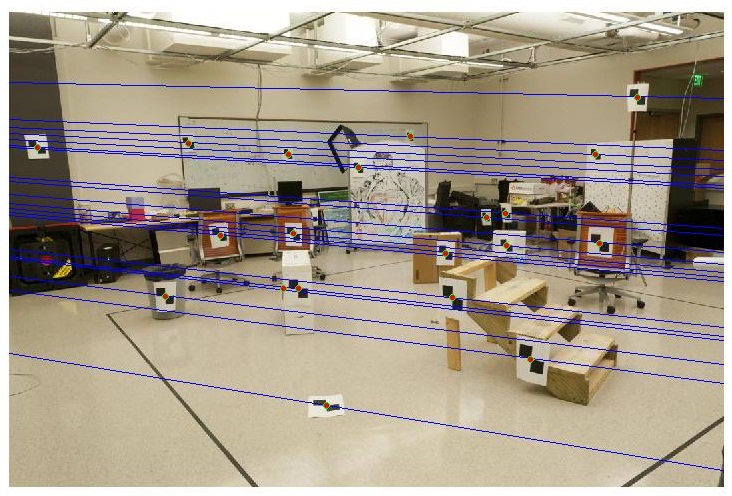
When normalized coordinates are used, we see that we obtain very reliable correspondences.
Inlier Keypoint correspondence:
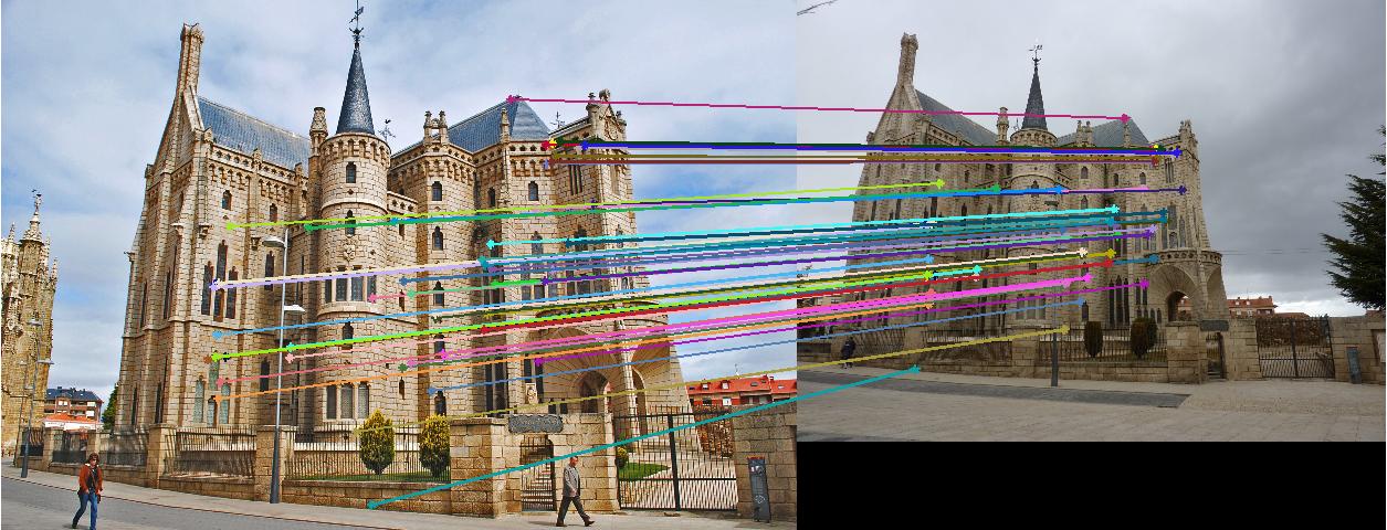
Epipolar lines:
The fundamental matrix estimated is also much more reasonable that the one obtained without normalized coordinates.