Project 3 / Camera Calibration and Fundamental Matrix Estimation with RANSAC
This project covers computing a camera projection matrix, estimating the fundamental matrix, and using RANSAC to estimate the fundamental matrix for an image pair. These concepts are important for understanding camera and scene geometry.
I. Camera Projection Matrix
To calculate the camera projection matrix, I used the homogeneous linear system approach discussed in class. I found the least squares solution for the given scene with known geometry, meaning a known 3D location mapped to known 2D image coordinates. This solution corresponds to the unknown camera parameters, a 3 by 4 matrix.
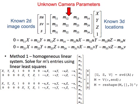
Fig. 1: Formula for least squares solution, taken from Lecture 13
To recover the camera center, I found -Q-1 m4, where Q is K * R, K is the 3x3 intrinsic matrix, and R is the 3x3 rotation matrix. The results of the camera projection matrix and camera center calculation are shown below.
The projection matrix is:
    0.4583   -0.2947   -0.0140    0.0040
   -0.0509   -0.0546   -0.5411   -0.0524
    0.1090    0.1783   -0.0443    0.5968


The total residual is: <0.0445>

The estimated location of camera is: <-1.5127, -2.3517, 0.2826>
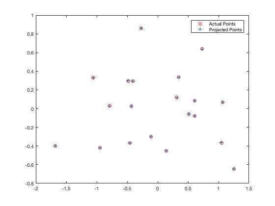
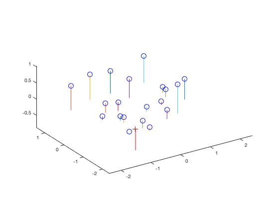
Fig. 2 (left): Camera projection matrix with total residual of 0.0445. Fig. 3 (right): Camera center with estimated location of (-1.5127, -2.3517, 0.2826).
II. Fundamental Matrix Estimation
I used an 8 point series of equations to estimate the fundamental matrix based on the set of points A and B. I first formulated a homogeneous linear equation, then used the Singular Value Decomposition (SVD) (similar to that used for the least squares solution) to find U, S and V making up the matrix of linear equations. The solution to this equation is of full rank, so I estimated the rank 2 fundamental matrix by setting the smallest singular value in S to 0, thus generating S2. The SVD of the augmented values gives the final fundamental matrix estimation (shown below).
F_matrix =

   -0.0000    0.0000   -0.0019
    0.0000    0.0000    0.0172
   -0.0009   -0.0264    0.9995
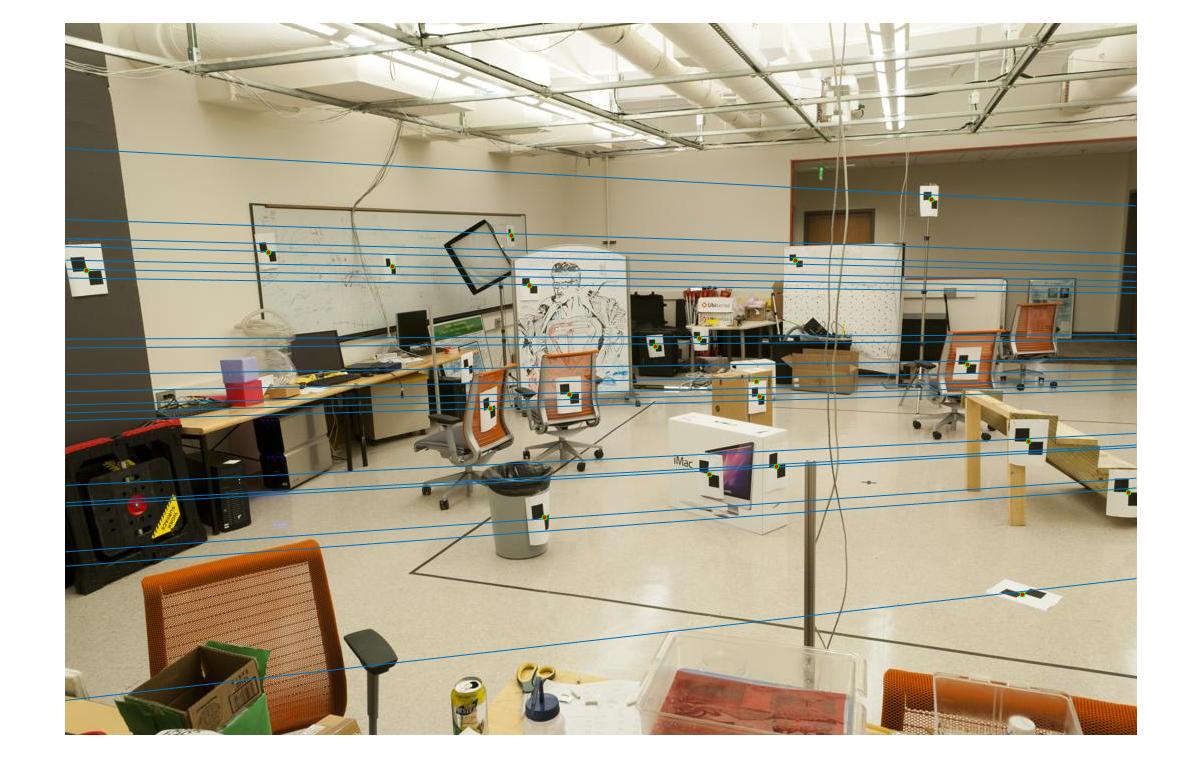
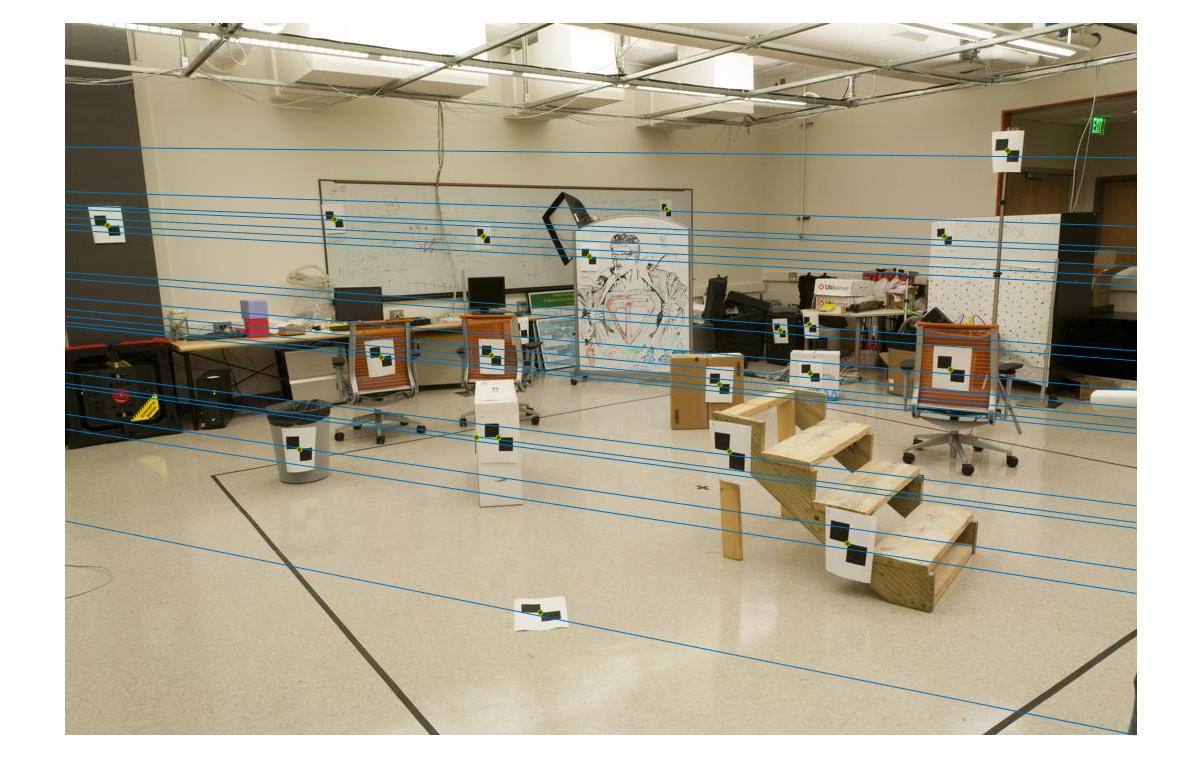
Fig. 4 and 5: Epipolar lines for fundamental matrix estimation.
Normalizing the Fundamental Matrix (Extra Credit)
I normalized the fundamental matrix by finding the average value (mean) of each set of points, determining the standard deviation of each set of points, and building a transformation matrix T. T was constructed by multiplying the product of the square root of two divided by a scale based on the standard deviation by a matrix with cu and cv being the left and middle most points. Cu and cv are the mean coordinates of Points A and Points B respectively. Once I had found the normalized fundamental matrix, I used my transformation matrix T to adjust the fundamental matrix so it could operate on the original pixel coordinates. The results of my normalization were more accurate than without normalization. Zooming in on the images shows that the epipolar lines go directly through the points when normalized, whereas they are slightly off the points otherwise.
F_matrix =

   -0.0000    0.0000   -0.0023
    0.0000   -0.0000    0.0184
   -0.0000   -0.0248    0.5274
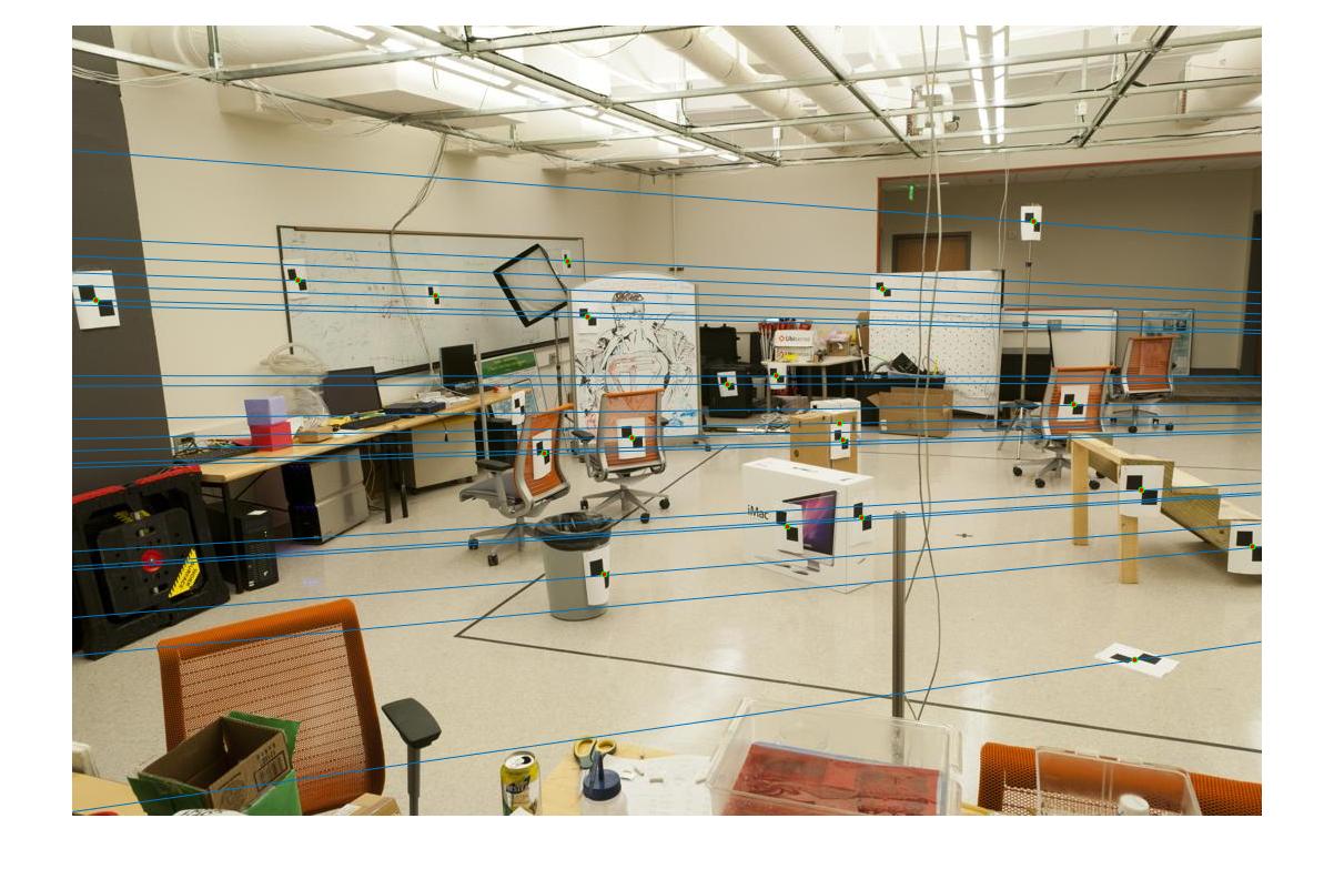

Fig. 6 and 7: Epipolar lines for normalized fundamental matrix estimation on original image.
III. Fundamental Matrix with RANSAC
This part of the project dealt finding the fundamental matrix using RANSAC for a set of images with unreliable point correspondences. For the RANSAC algorithm, I used p = 0.99 (chance of success required), e = 0.5 (outlier ratio), s = 8 (for the 8-point algorithm), and N = log(1 - p)/log(1 - (1 - e)s). I completed "N" iterations in which I randomly sampled the matches provided, determined the fundamental matrix for those samples, scored the fundamental matrix, determined the number of successful matches, and returned the best match. The best match was determined by finding the number of matches (in the scoring process) and returning the fundamental matrix and related inliers that resulted in the most matches. Several examples of this algorithm working are shown below.
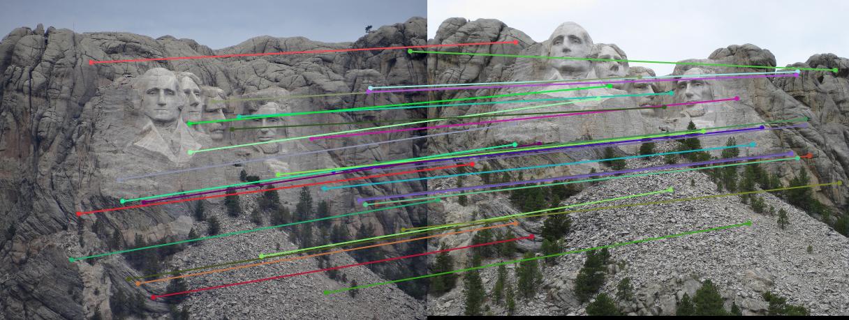
Fig. 8: Mount Rushmore matches with 30 samples.
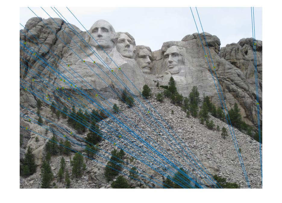
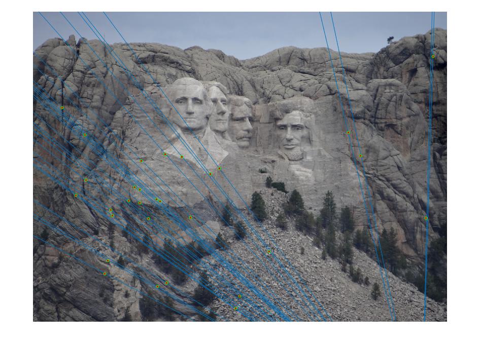
Fig. 9 and 10: Epipolar lines for Mount Rushmore image.
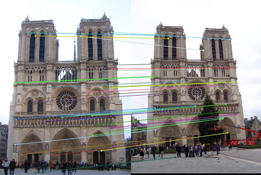
Fig. 11: London Tower with 30 matches.
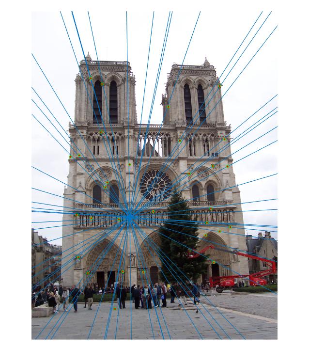
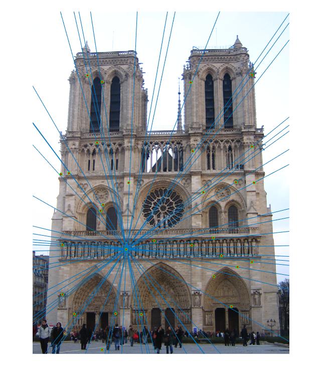
Fig. 12 and 13: Epipolar lines for London Tower image.
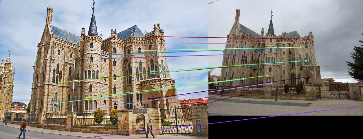
Fig. 14: Gaudi pair with 15 matches shown.
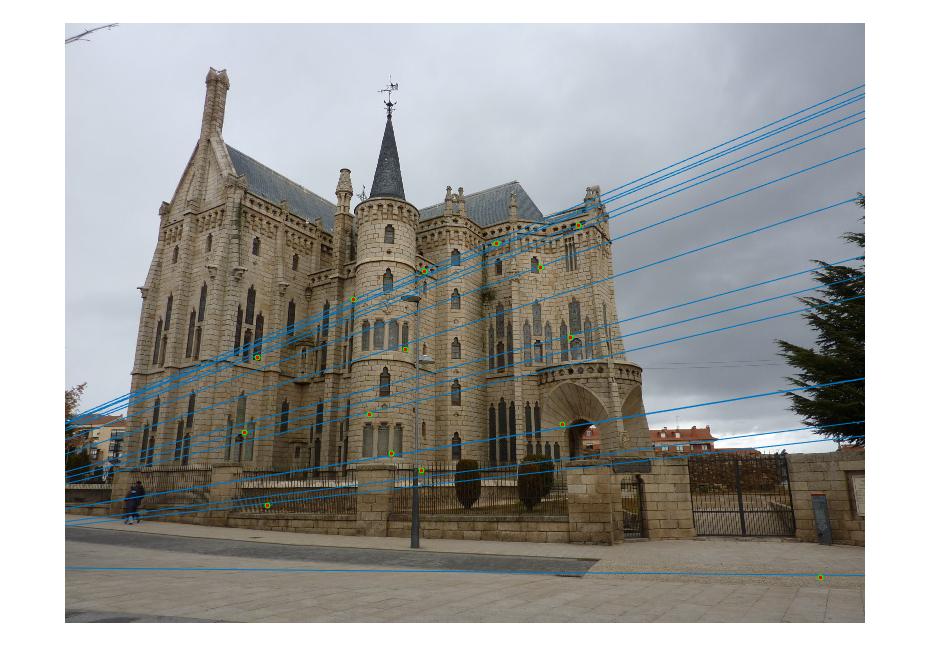
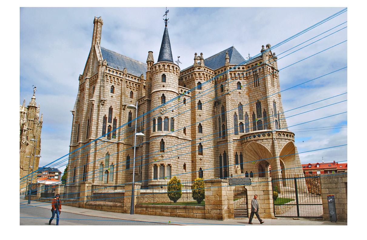
Fig. 15 and 16: Epipolar lines for Gaudi image.
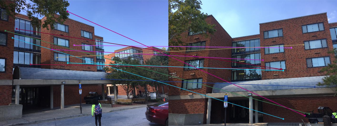
Fig. 17: Woody's with 10 matches shown. The algorithm had some trouble with this image.
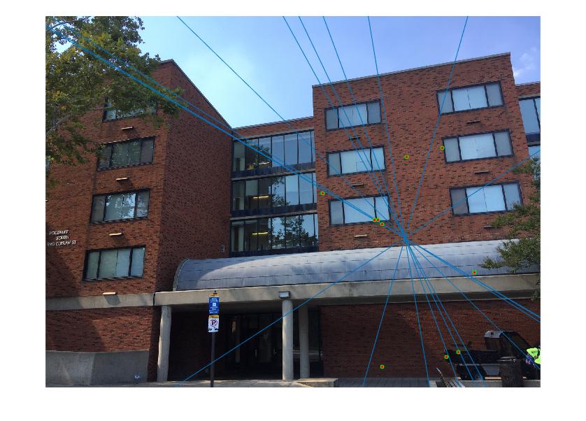
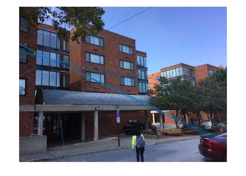
Fig. 18 and 19: Epipolar lines for Woody's building.