Project 3 / Camera Calibration and Fundamental Matrix Estimation with RANSAC
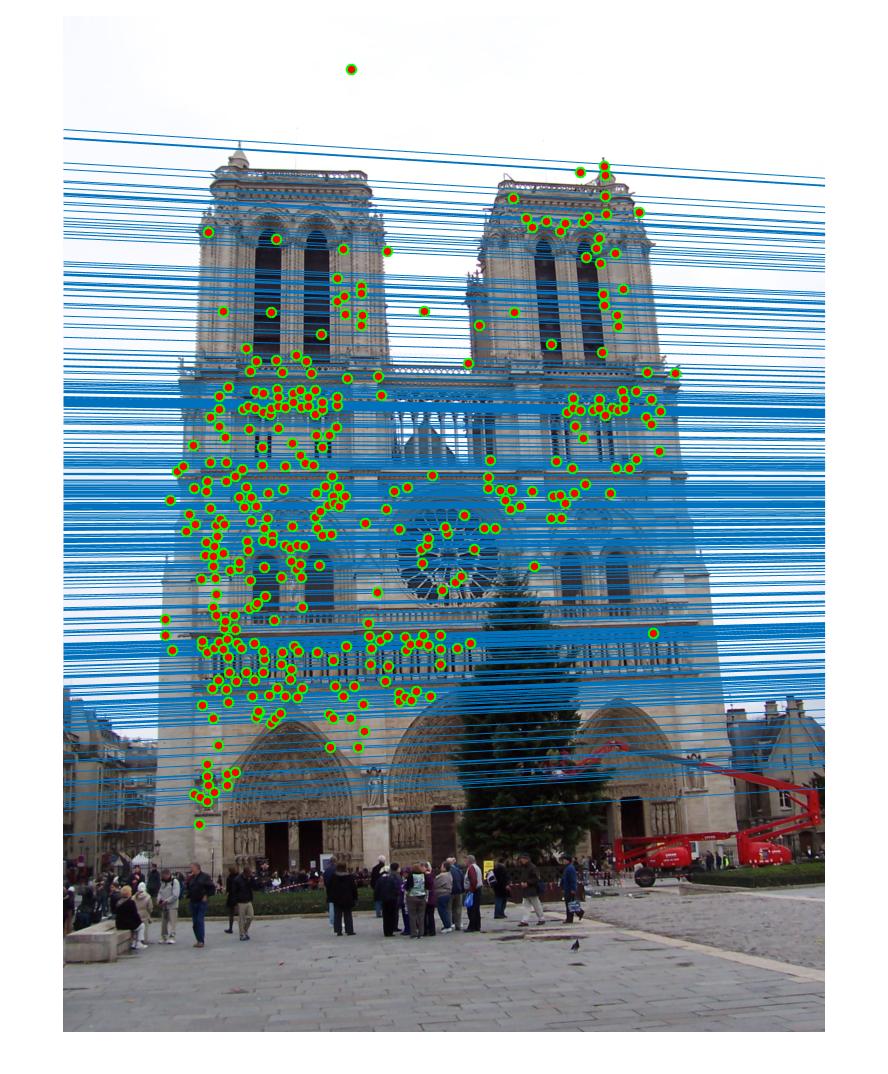
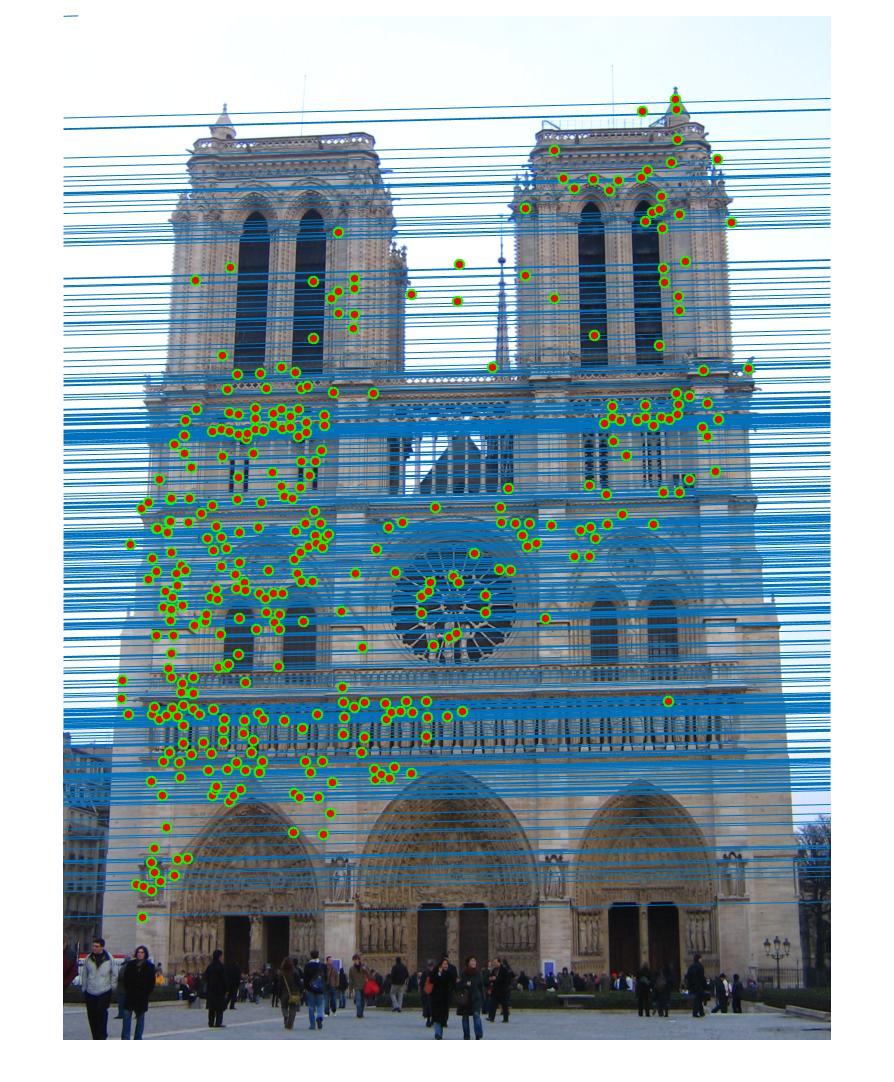
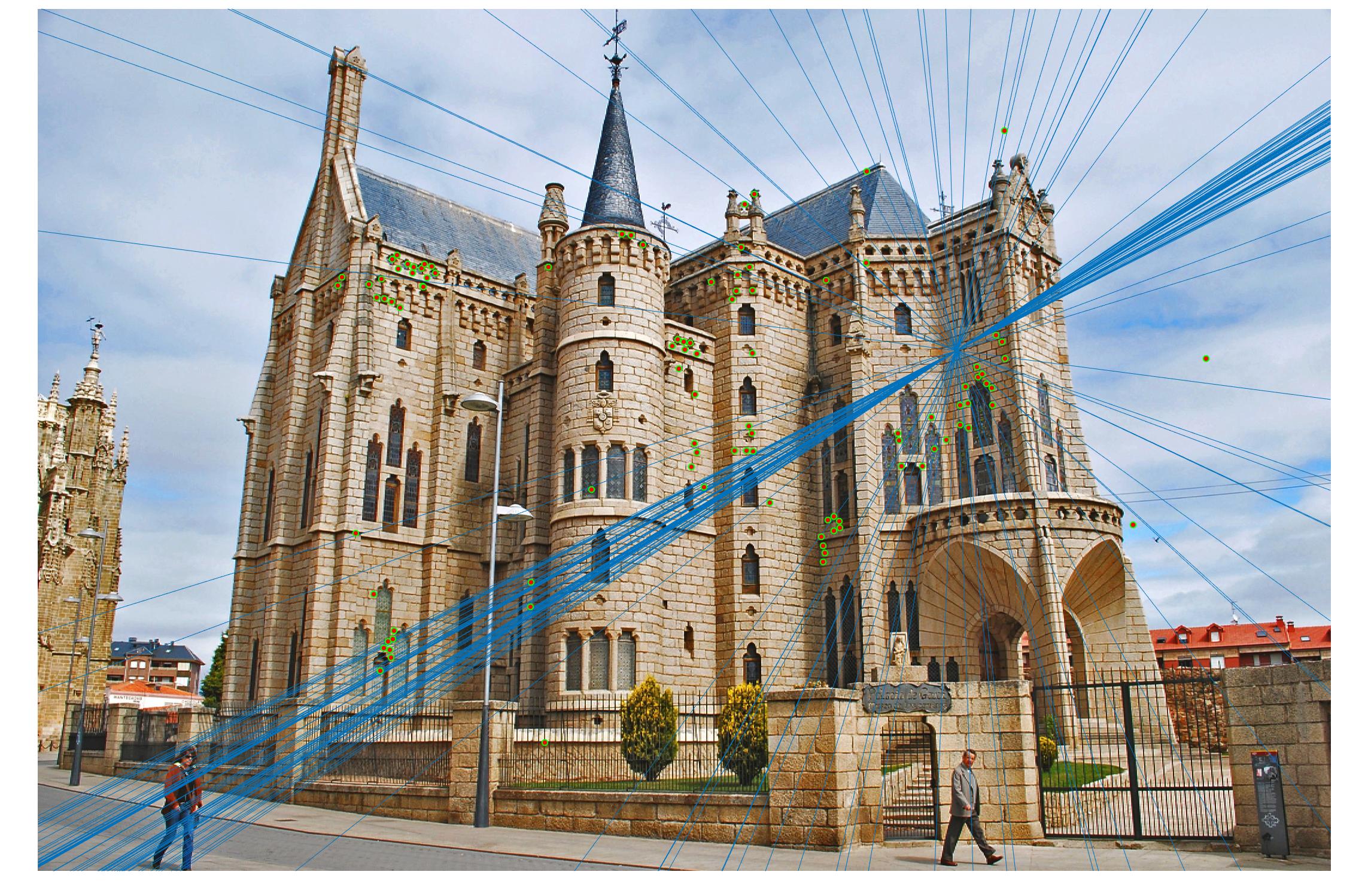
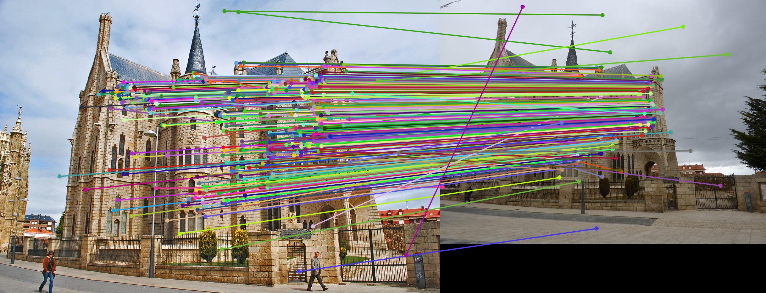
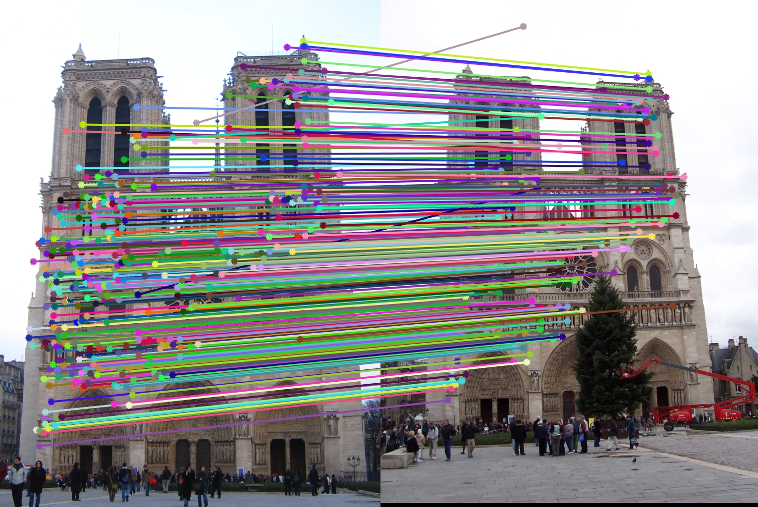
Example estimation of epipolar lines and matching points.
This project has three parts:
- Camera Projection Matrix.
- Fundamental Matrix Estimation.
- Fundamental Matrix with RANSAC.
The picture above shows an example estimation of epipolar lines and matching points obtained in part 3. By using RANSAC, I am able to reject most of the bad matches and calculate a good fundamental matrix. Below will discuss the results of the three parts and how the algorithms are designed to produce a good result.
Part 1: Camera Projection Matrix
For each 2D and 3D point pair, I can obtain two equations, from which a matrix equation "A * M = 0" is constructed. Then, I use SVD to solve the equation for M, which is the camera projection matrix.
The values calculated from pts2d-norm-pic_a and pts3d-norm:
The projection matrix is:
0.4583 -0.2947 -0.0140 0.0040
-0.0509 -0.0546 -0.5411 -0.0524
0.1090 0.1783 -0.0443 0.5968
The total residual is: <0.0445>
The estimated location of camera is: <-1.5127, -2.3517, 0.2826>
The values calculated from pts2d-pic_b and pts3d:
The projection matrix is :
0.0069 -0.0040 -0.0013 -0.8267
0.0015 0.0010 -0.0073 -0.5625
0.0000 0.0000 -0.0000 -0.0034
The total residual is: <15.5450>
The estimated location of camera is: <303.1000, 307.1843, 30.4217>.
Part 2: Fundamental Matrix Estimation
The approach is similar to part 1 in that I need to solve "A * f = 0" for f where f is the linearly reshaped fundamental matrix. However, I need to enforce singularity constraints by resolving det(F) = 0 using SVD as well. In addition, I normalize the point pairs in this step, which significantly improves the result of RANSAC in part 3. I will discuss the extra credit later.
The calculated fundamental matrix for the base image pair (pic_a.jpg and pic_b.jpg) is:
F_matrix =
0.0000 -0.0000 0.0007
-0.0000 0.0000 -0.0054
0.0000 0.0074 -0.1716
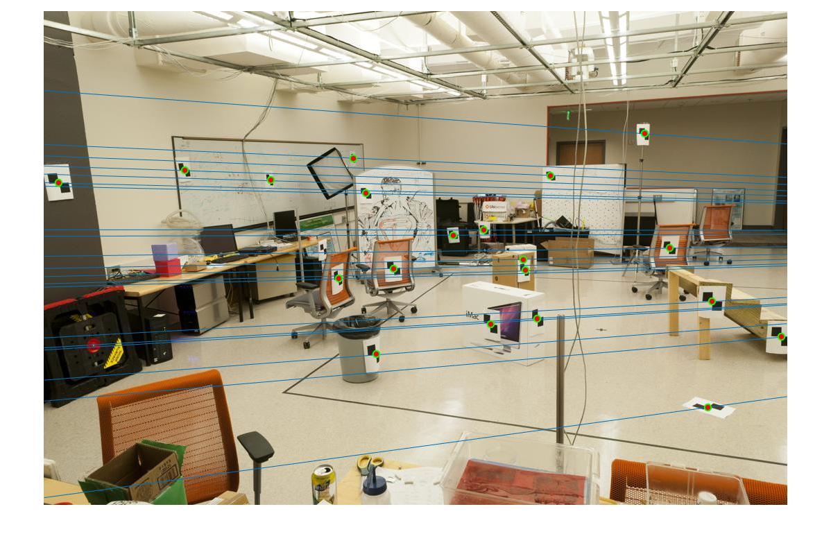
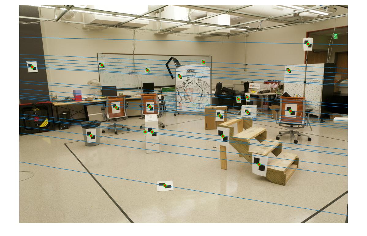
The epipolar lines are shown below.
Part 3: Fundamental Matrix with RANSAC
There are three major steps in each loop of my implementation of RANSAC:
- Randomly pick 8 point pairs.
- Estimate a fundamental matrix with the 8 points.
- Calculate abs(a * F * transpose(b)) where a and b are homogeneous point pair and keep the results less than a threshold as inliers.
After all the iterations, use the fundamental matrix which generates the most inliers.
In the above steps, there are two important parameters in RANSAC:
- Number of iterations: I set it to 5000. Although it takes longer time to do more iterations, it increases the probablity of picking better point pairs which generate a better fundamental matrix.
- Threshold for rejecting outliers: I set it to 0.045. This number is primarily a empirical number that works the best with 5000 iterations. 0.05 is good enough but it can not be less than 0.04
Extra credit: Points Normalization
I use the following matrix operation to normalize the points.
I use a single transfrom matrix for points in both pictures. Therefore, the calculation of scaling factor and offset is all based on the points in both images. The offset c_u and c_v are the mean of the coordinates. I use two different scaling factor for the two dimensions of points, which are s_u and s_v. They are the reciprocal of the standard deviation of the points relating to the means.
The code that calculates the transform matrix is as following.
c_u = mean([Points_a(:,1); Points_b(:,1)]);
c_v = mean([Points_a(:,2); Points_b(:,2)]);
s_u = 1 / std([Points_a(:,1) - c_u; Points_b(:,1) - c_u]);
s_v = 1 / std([Points_a(:,2) - c_v; Points_b(:,2) - c_v]);
Points_a = [Points_a, ones(n,1)];
Points_b = [Points_b, ones(n,1)];
T = [s_u, 0, 0; 0, s_v, 0; 0, 0, 1] * [1, 0, -c_u; 0, 1, -c_v; 0, 0, 1];
The transform matrix is applied to each point pair.
Points_a(i,:) = T * Points_a(i,:)';
Points_b(i,:) = T * Points_b(i,:)';
At the end, the original fundamental matrix can be calculated from the fundamental matrix obtained from the normalized point pairs
F_matrix_orig = T' * F_matrix_norm * T;
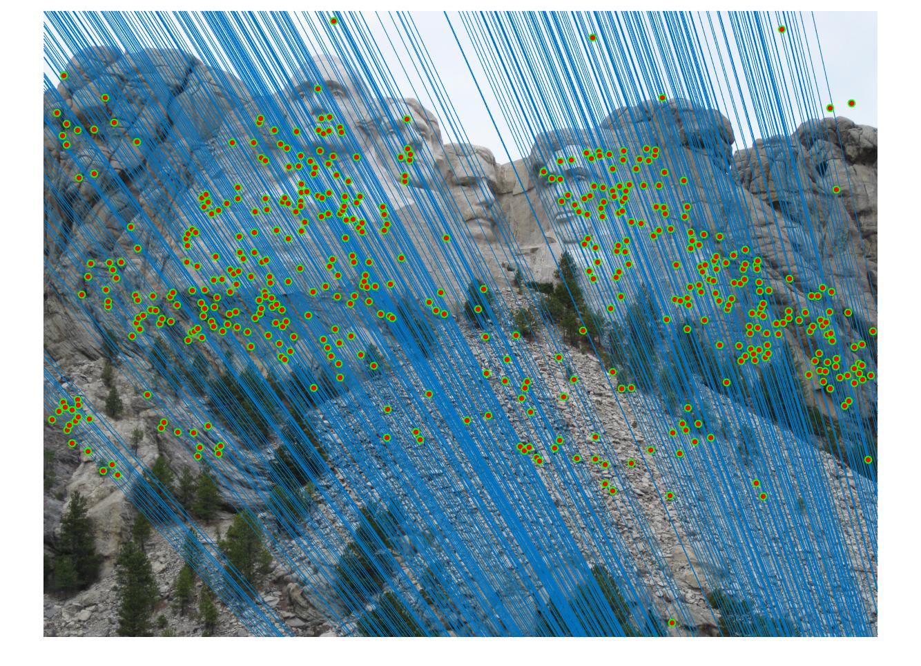
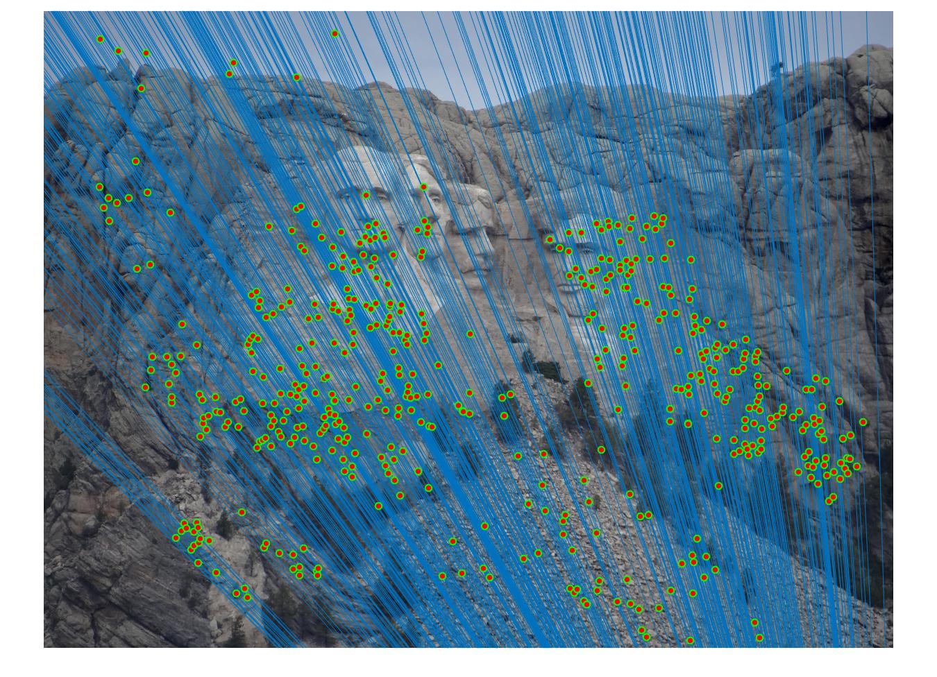
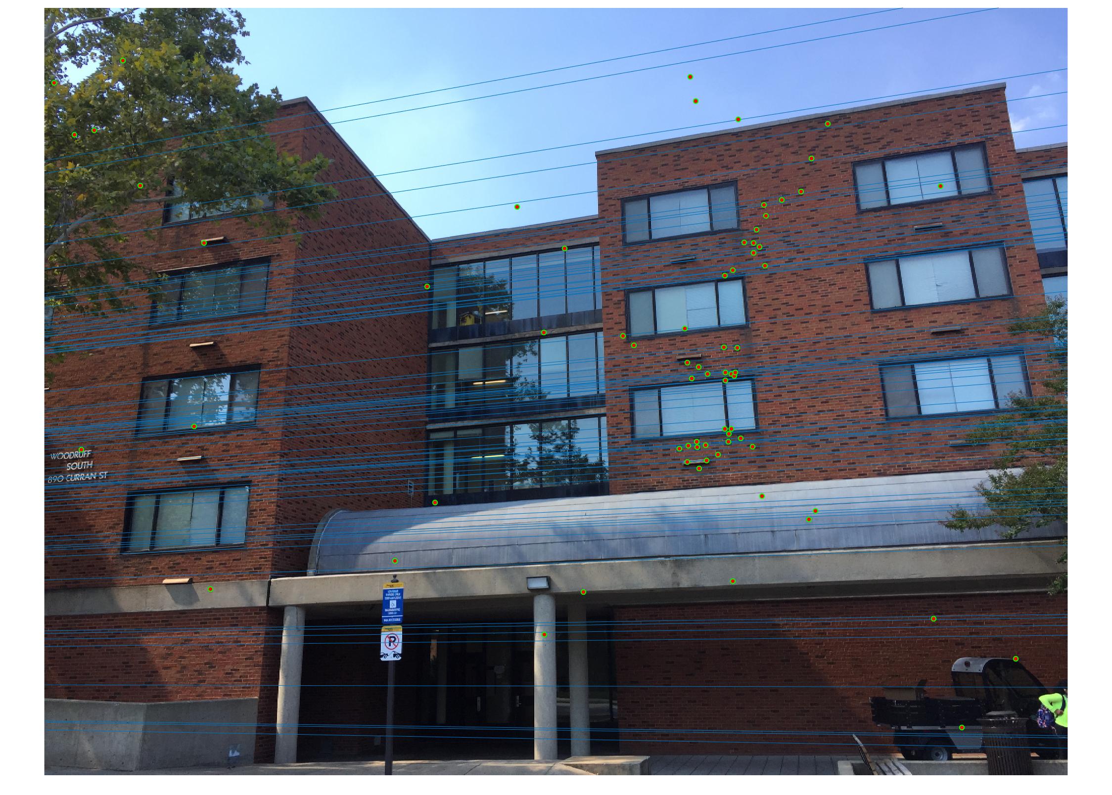
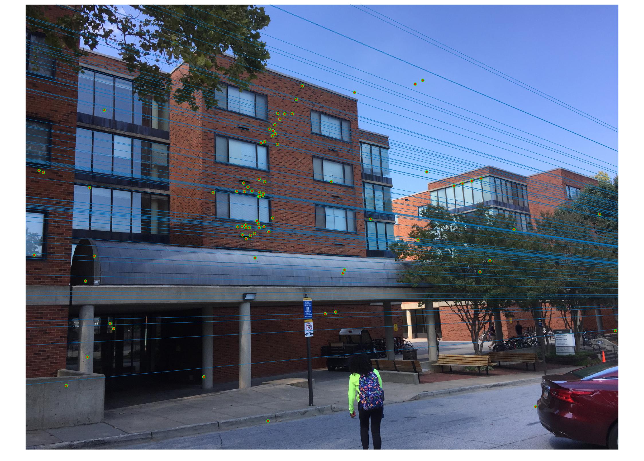
Comparison between results before and after normalization
Before

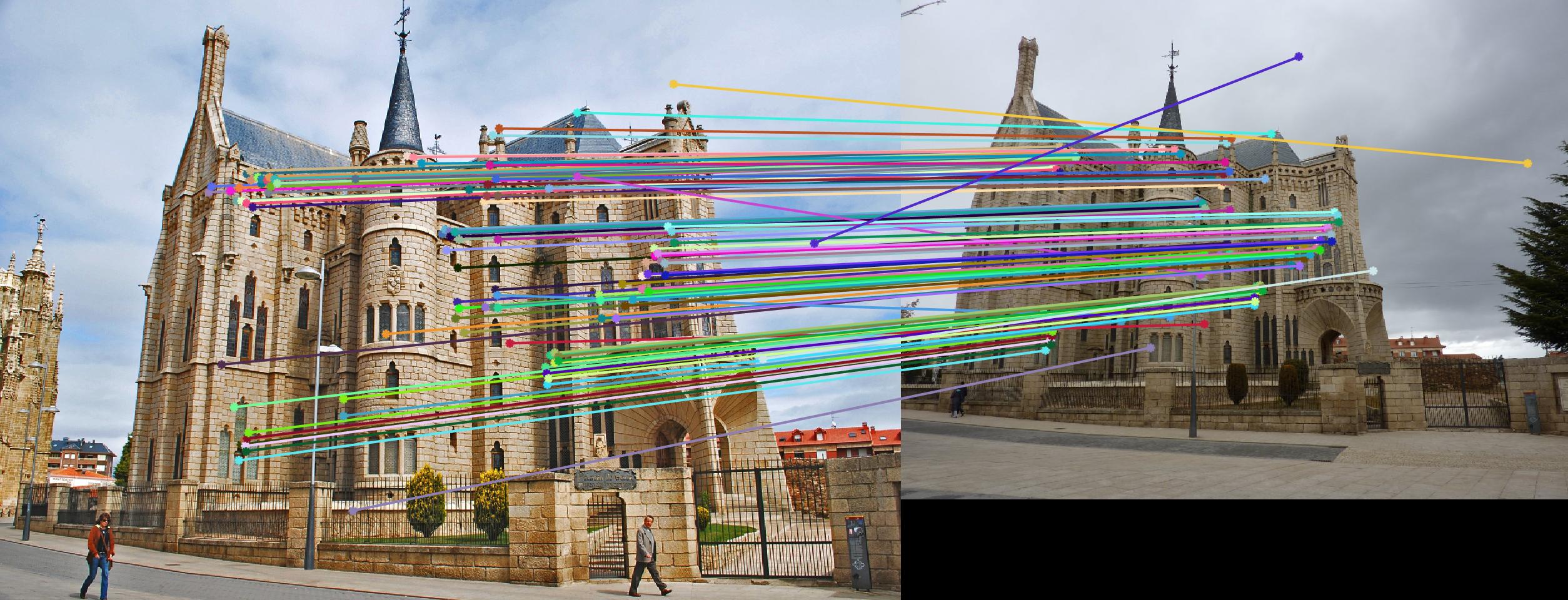
|
After
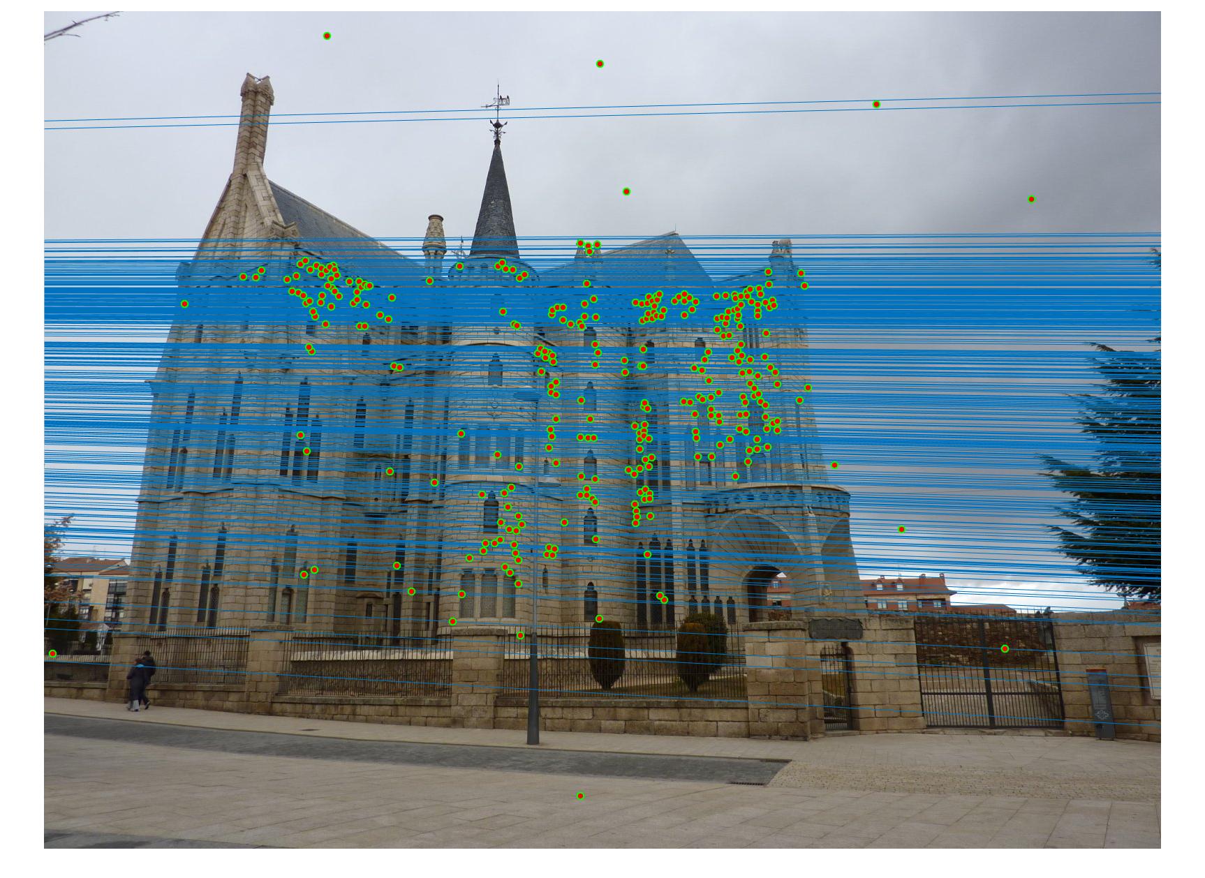
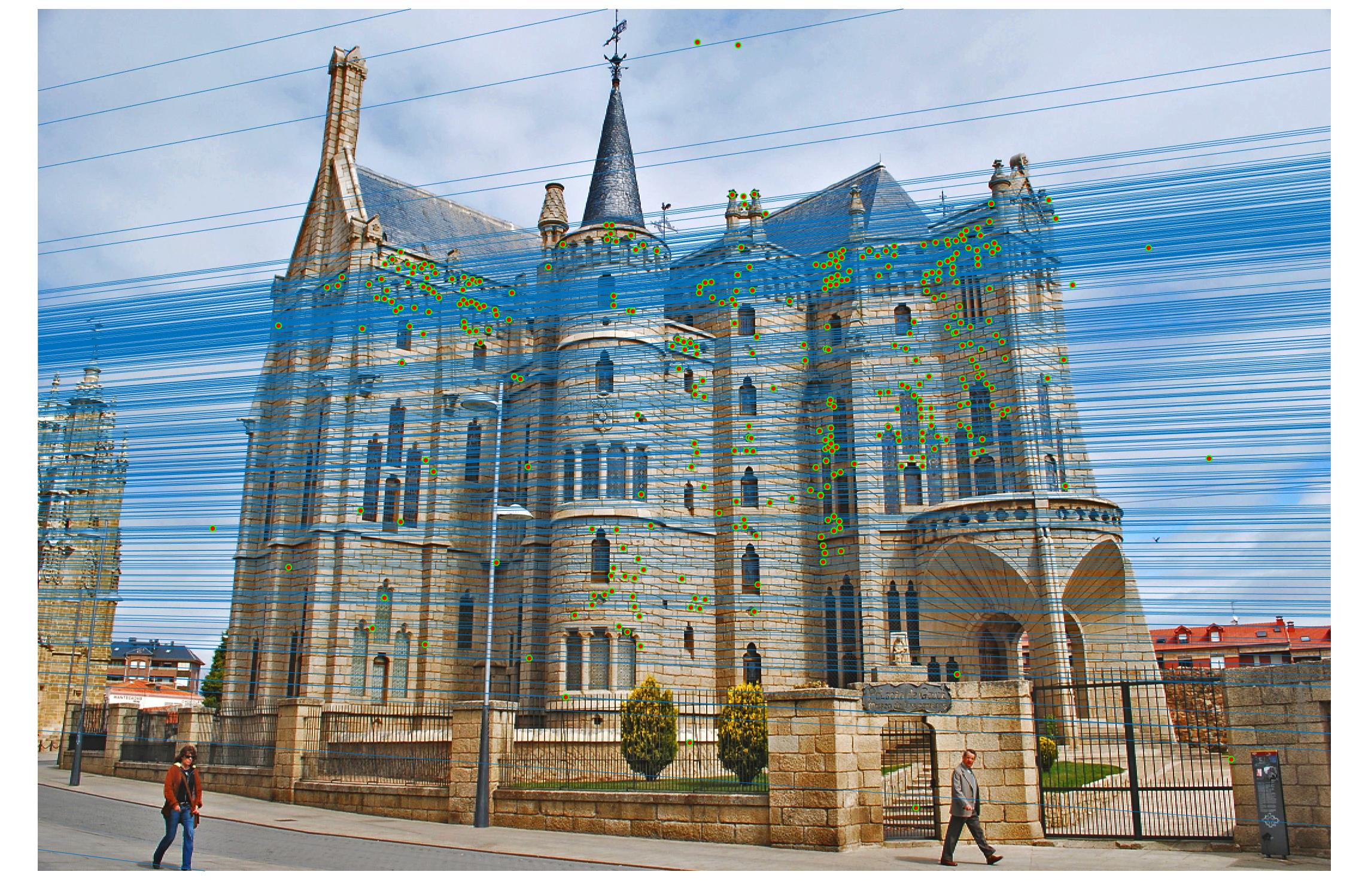
|
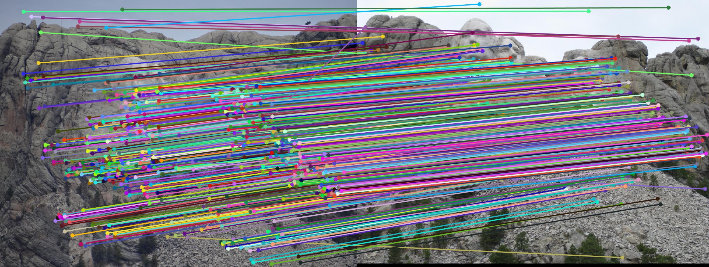
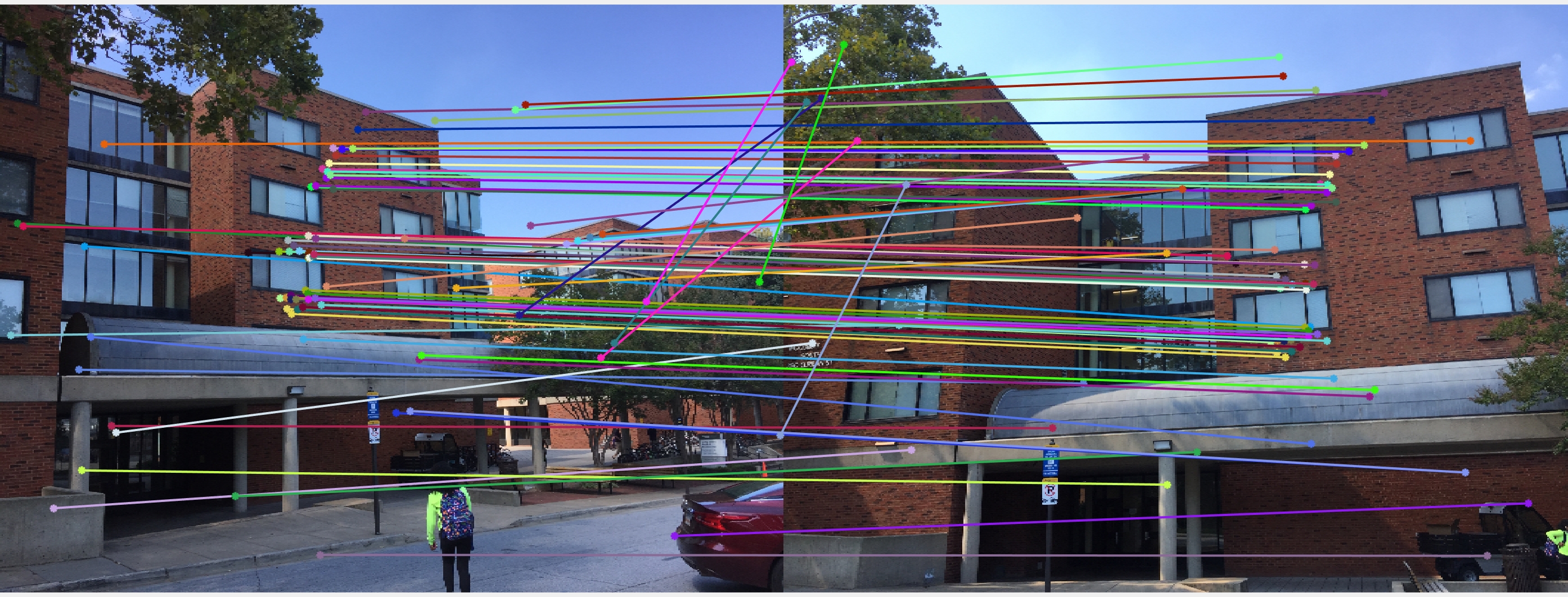
Results with Normalization
|
|
|
|
|
There are a lot of matching points shown in the images above. A further step could be done to filter out some of the bad matches shown above. We could order the inliers with the value calculated from abs(a * F * transpose(b)) and pick certain number of matches with the smallest calculated value and use them to display the epipolar line and point matches.