Daniel Cohen

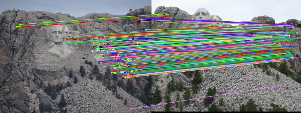
Filtered SIFT matches for Mount Rushmore image pair.

Camera Calibration

To compute the camera calibration matrix, the correspondence between real-world 3D point coordinates and projected 2D coordinates in the image is used. This data is collected ahead of time, and provided as input to the function. The function loads this data into a specially-constructed matrix, and computes the null-space using SVD. The resulting null-space vector is reshaped into a 3x4 matrix which describes how 3D points are mapped to 2D image coordinates. The matrix is then normalized. In this case, the matrix was also multipled by -1 to match the signs with the expected output. This does not affect the matrix, since it is normalized. Using the provided data, the output is: $$ \begin{bmatrix} -0.4583 & 0.2947 & 0.0140 & -0.0040 \\ 0.0509 & 0.0546 & 0.5411 & 0.0524 \\ -0.1090 & -0.1783 & 0.0443 & -0.5968 \end{bmatrix} $$ Comparing the expected locations to the locations predicted by the matrix, we get the following visualization:

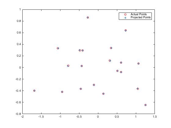
Clearly, the calibration error is extremely small, and more importantly, non-systematic. In other words, the errors for each point appear to be random noise, and therefore not the result of an incorrectly computed matrix. This is confirmed by the small residual, 0.0445.

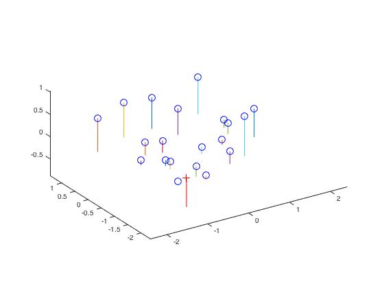
Using the calibration matrix, we can estimate the location of the camera in the world, by inverting the first three columns and multiplying it by the fourth column as a vector. Using this technique, the camera center is estimated to be: $$ \begin{bmatrix} -1.5127 & -2.3517 & 0.2826 \end{bmatrix} $$

If we visualize the result, it is clear that this location matches our qualitative interpretation of the scene:

Computing the Fundamental Matrix

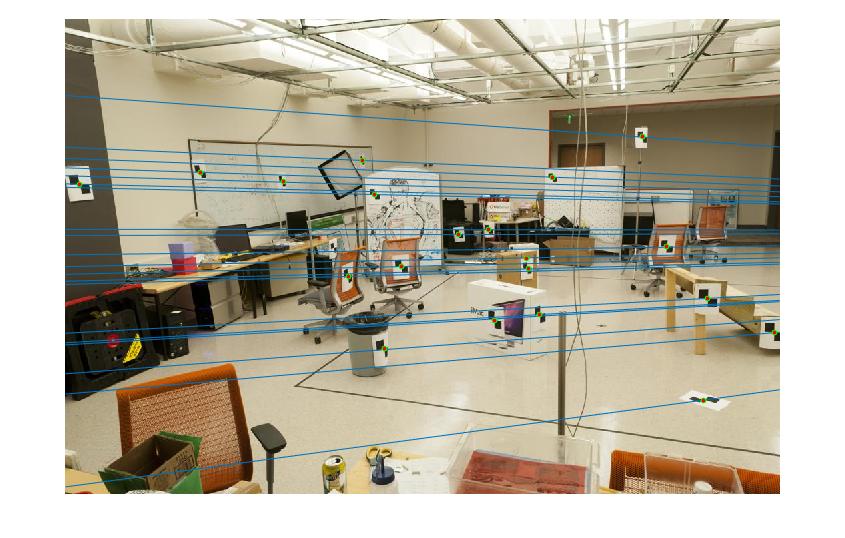
Computing the Fundamental Matrix is a similar process to computing the Calibration Matrix. After all, they're both regression. However, it requires more processing to get a satisfactory result. In order to get a good condition number when we factor the matrix with SVD, we first normalize the input points. This is relatively simple; we simply shift the centroid of the points to (0, 0) and then adjust the coordinates so the mean distance of the points from the origin is $\sqrt{2}$. We then represent this transformation as a product of scaling and transformation matricies: $$ T = \begin{bmatrix} scale & 0 & 0 \\ 0 & scale & 0 \\ 0 & 0 & 1 \end{bmatrix} \cdot \begin{bmatrix} 1 & 0 & -mean_x \\ 0 & 1 & -mean_y \\ 0 & 0 & 1 \end{bmatrix} $$ We then use the normalized values to compute a scaled fundamental matrix, and then de-normalize to get the real matrix as follows: $$ T = T'^T \cdot F_{norm} \cdot T $$ The result of this algorithm is that the Fundamental matrix has much better numerical stability and the epipolar lines are much more accurate:

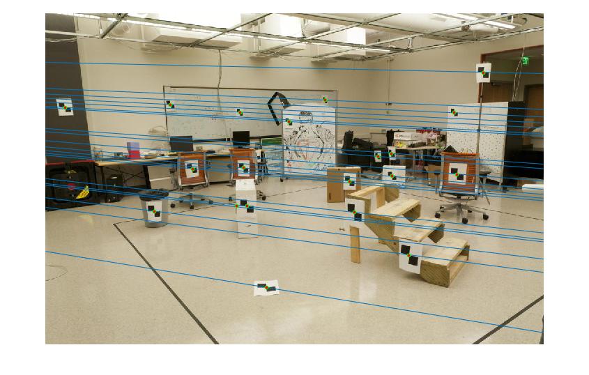Every epipolar line goes almost exactly through the correct point, which is the desired result.

Filtering SIFT Matches

Using the Fundamental Matrix we computed. We can filter out spurrious SIFT matches that don't correspond to the epipolar geometry discovered above. This requires a RANSAC technique. This RANSAC implementation runs for 1,000 iterations, using a sample size of 10, two more than the minimum number of points needed to compute a Fundamental Matrix. It considers any point to be an inlier if the error is less than 0.01.

Eight points are chosen at random, and then used to estimate a Fundamental Matrix. Then the number of inliers is counted by checking if the error is less than 0.1. The error is computed by leveraging the epipolar identity $x^TFx' = 0$. Since this expression should evaluate to 0 in a perfect world, this value is used to determine whether a point is an inlier or not.

Using this technique, we can plot the set of inliers with the lowest error for each image pair we explored in the previous project:

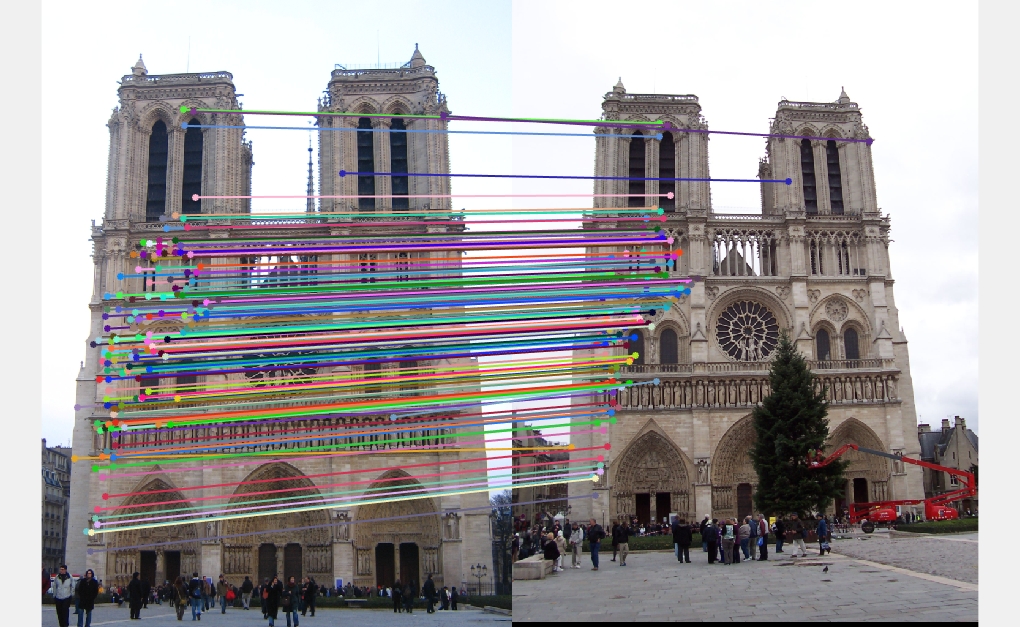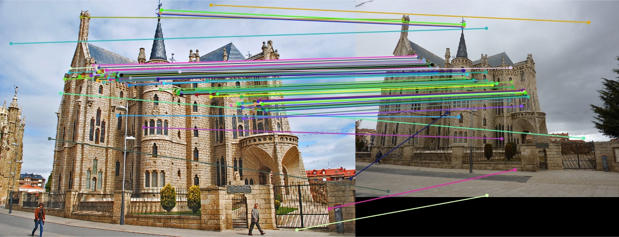Both the Mount Rushmore and Notre Dame pairs get perfect accuracy using this technique. However, Gaudi still performs a little worse. The most likely reason is that it has many more matches than either of the other two pairs. This means that more iterations would be required.