Project 3 / Camera Calibration and Fundamental Matrix Estimation with RANSAC
Part I: Camera Projection Matrix
This project is on camera and scene geometry. First we want to estimate the camera projection matrix from known 3d to 2d correspondence data. We do this through linear regression. When we compute the projection matrix we also get the camera center. The projection matrix is:
| 0.7679 |
-0.4938 |
-0.0234 |
0.0067 |
| -0.0852 |
-0.0915 |
-0.9065 |
-0.0878 |
| 0.1827 |
0.2988 |
-0.0742 |
1.0000 |
The total residual is: 0.0445. The estimated location of camera is: <-1.5126, -2.3517, 0.2827>
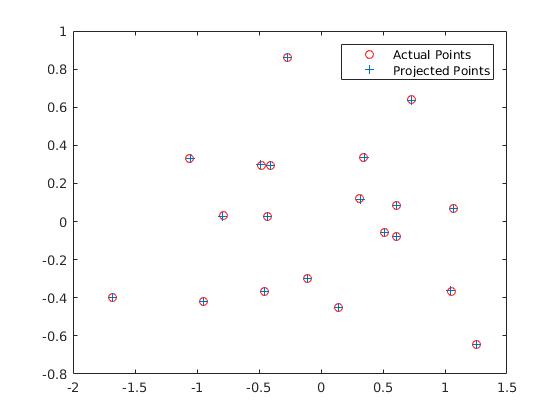
Comparison of actual and projected 3D points onto the 2D camera plane using the estimated projection matrix
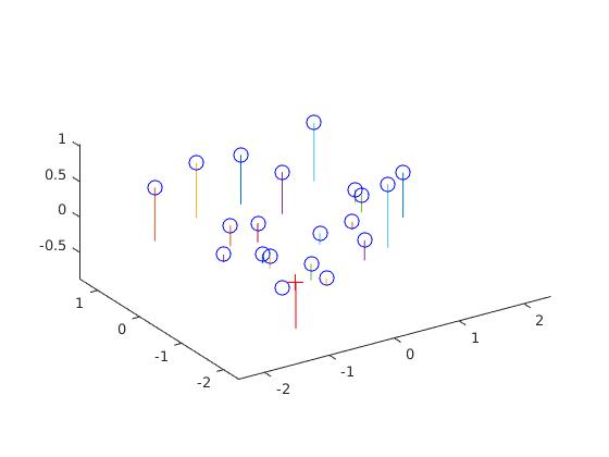
Position of camera center relative to the 3D positions of known object locations.
Part II: Fundamental Matrix Estimation
Now we estimate the funamdental matrix from a given set of known corresponding points. Again, we do this through linear regression (using SVD decomposition). We also make sure that the estimated fundamental matrix has less than rank 3 to ensure that the epipolar lines converge at one point. The estimated matrix is:
| -0.0000 |
0.0000 |
-0.0019 |
| 0.0000 |
0.0000 |
0.0172 |
| -0.0009 |
-0.0264 |
0.9995 |

|
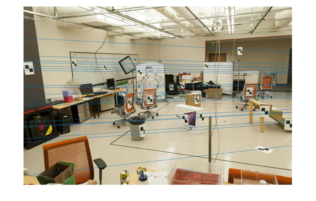
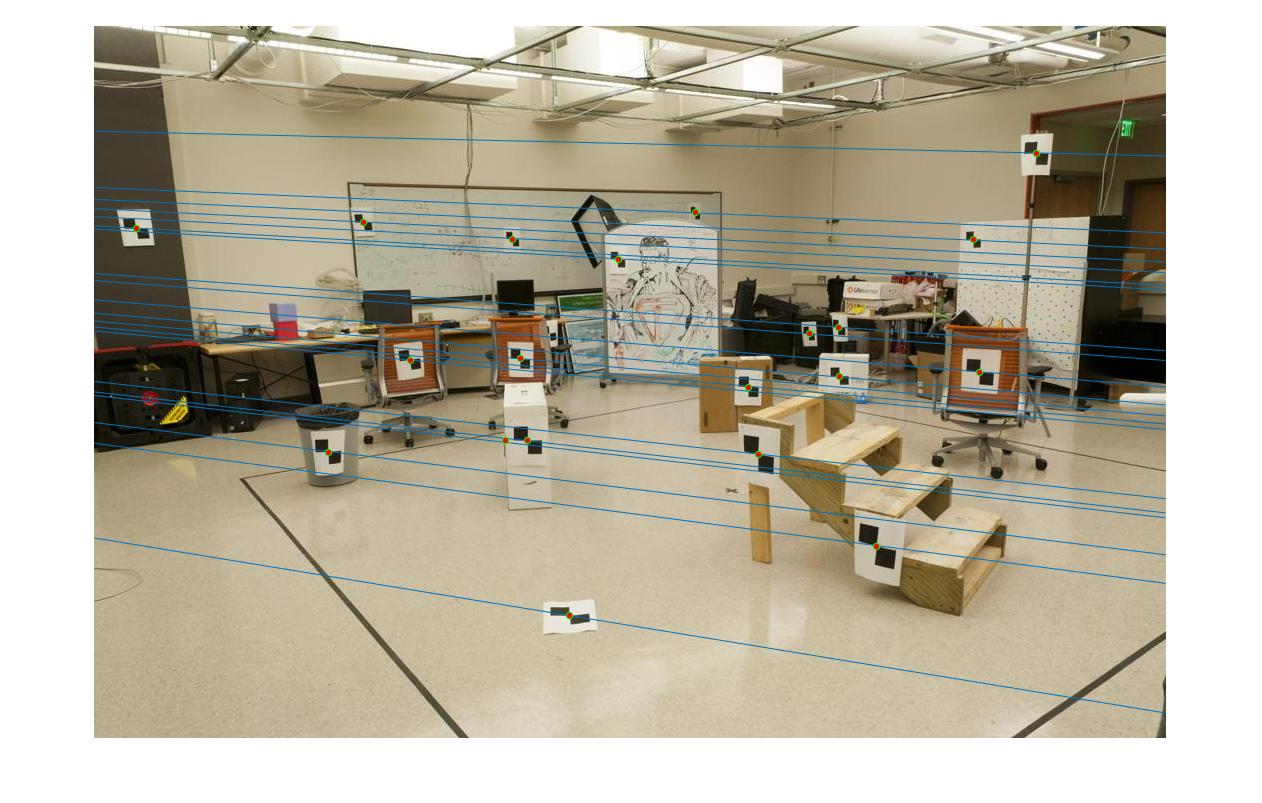
Epipolar lines drawn for the stereo images via the estimated fundamental matrix from known correspondences.
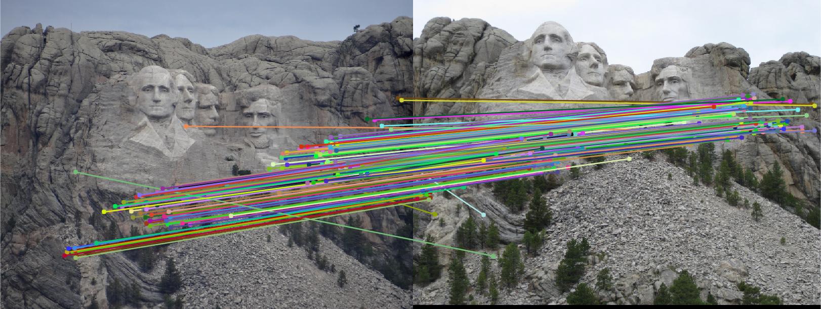
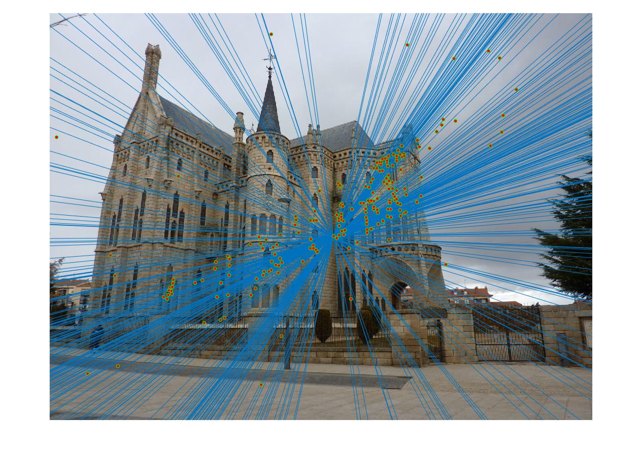
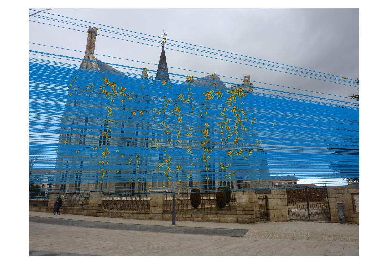
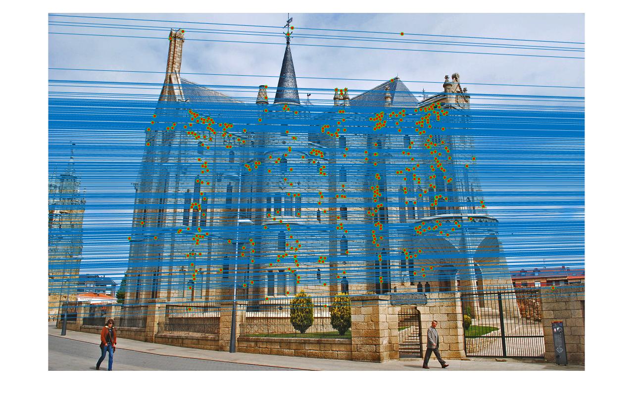
Part III: Fundamental Matrix with RANSAC
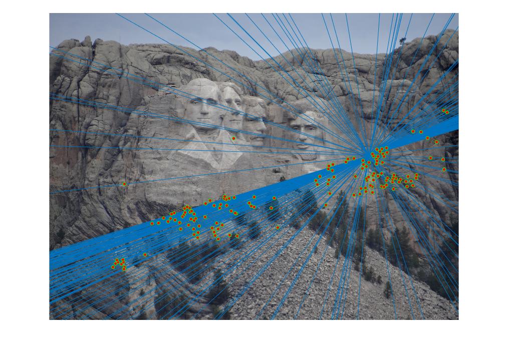
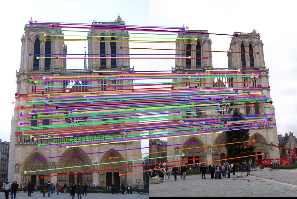
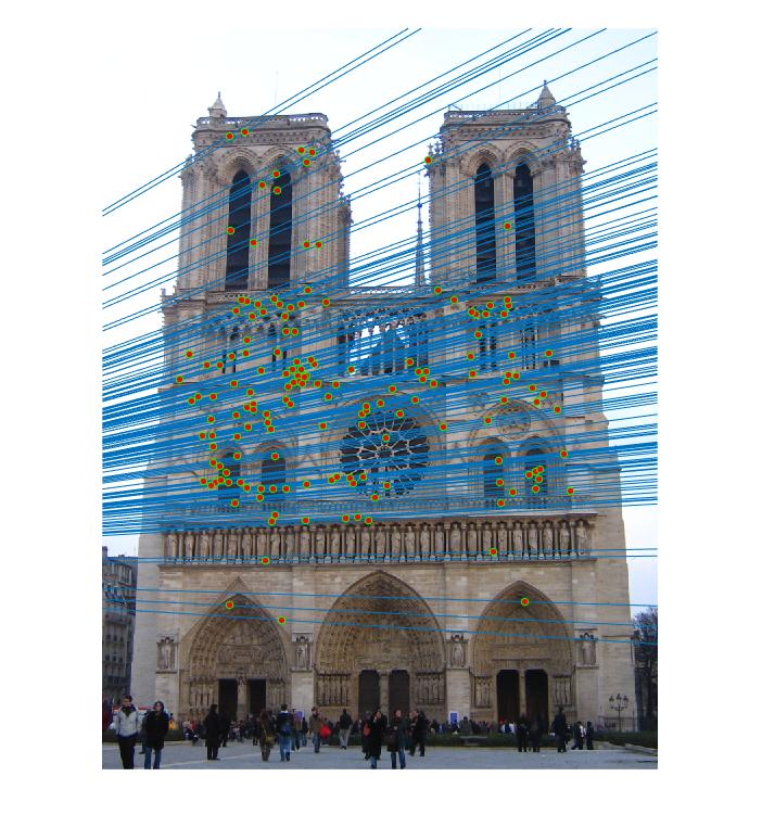
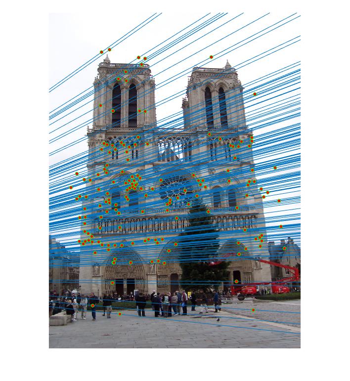
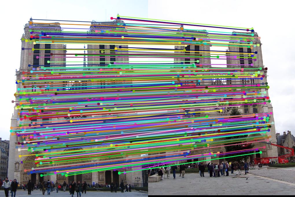
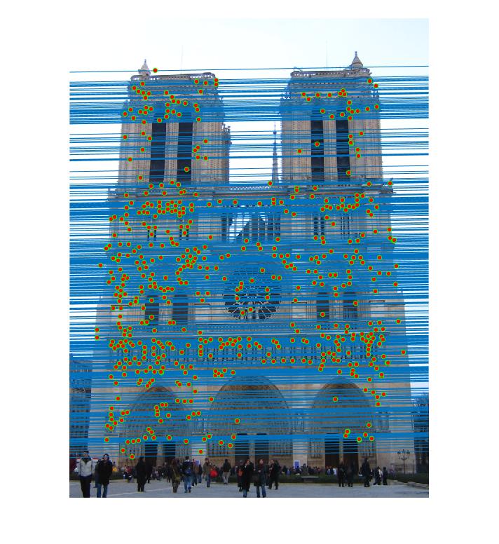
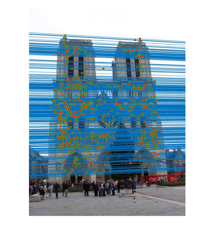
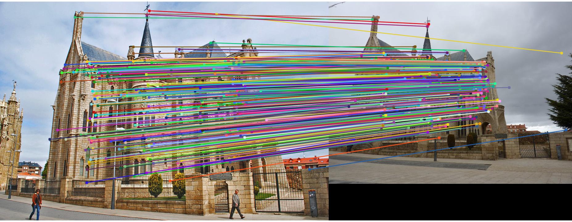
Now we use RANSAC to estimate the best fundamental matrix from SIFT features. To do this we sample a small batch of matches and calculate a fundamental matrix, then find the number of inliers. We keep doing this until we find a matrix with the highest number of inliers. There tend to be a few spurious matches, and only the Notre Dame's epipolar lines make sense.
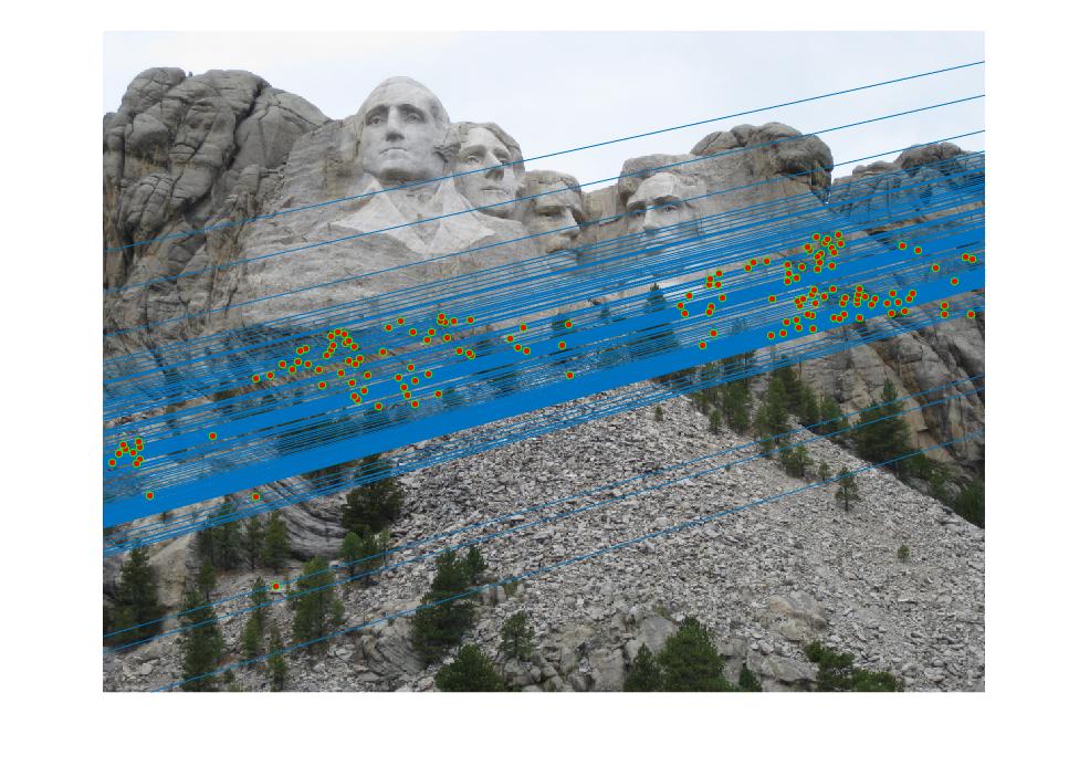
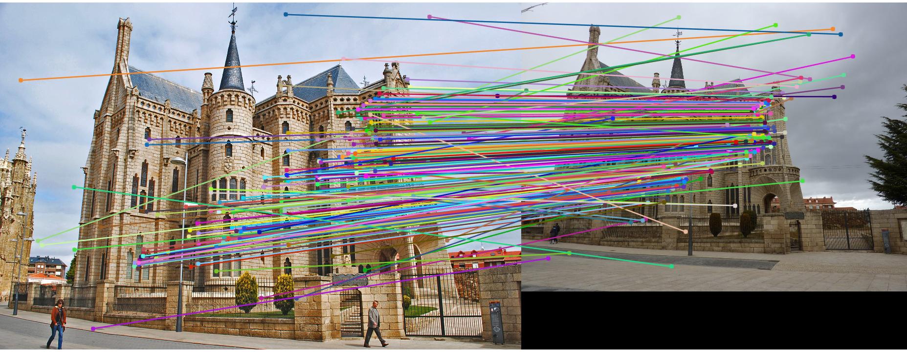
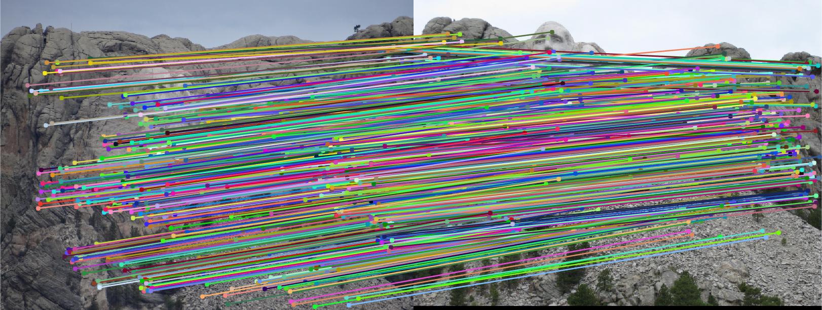
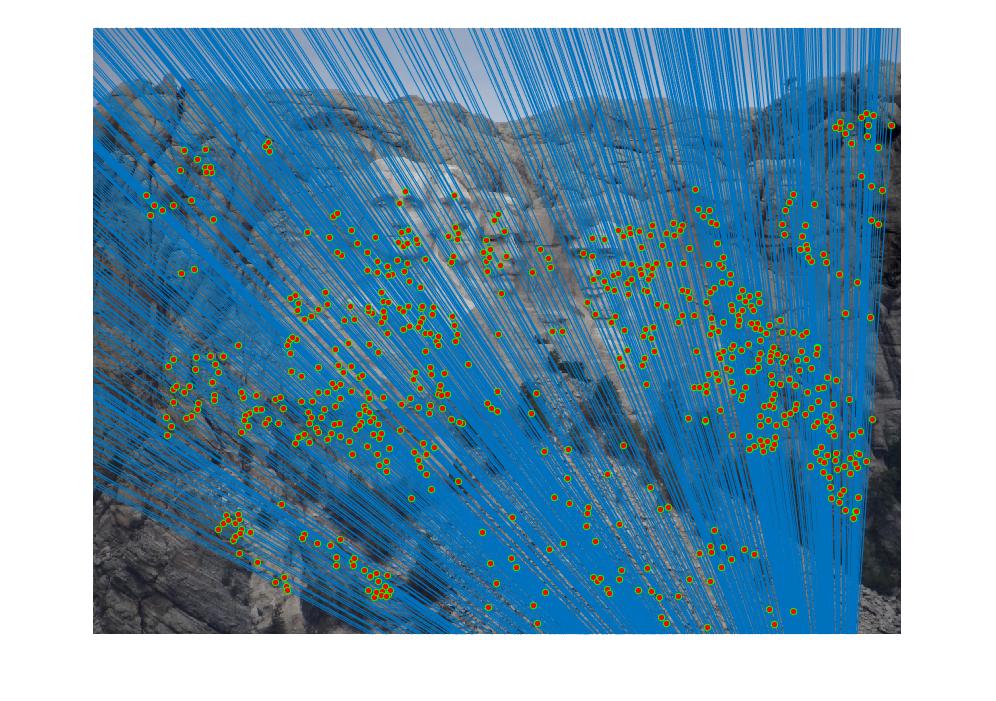
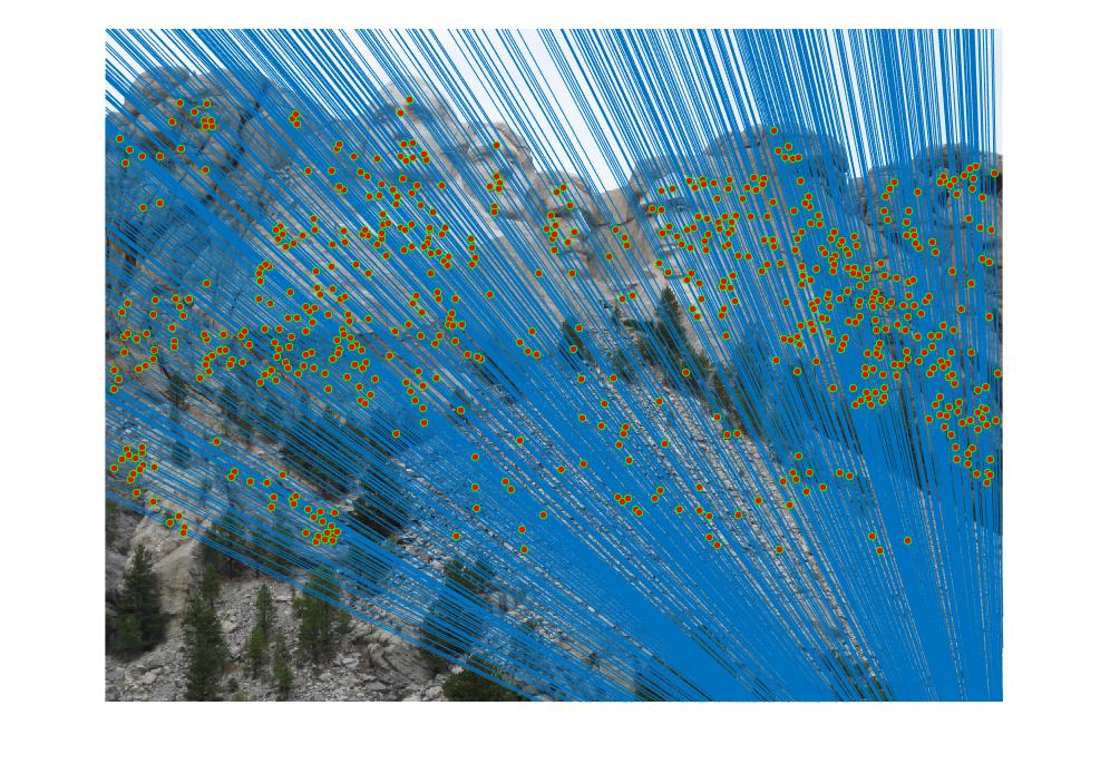
EXTRA: Normalized Fundamental Matrix with RANSAC
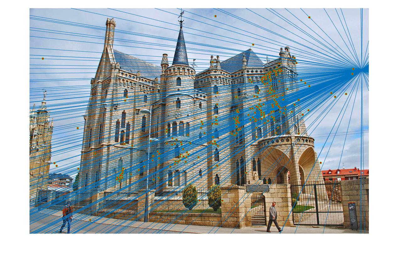
Before performing the estimation of the fundamental matrix, we normalize the coordinates. To do this we use the mean and standard deviation from each image to normalize the coordinates from the images seperately. The result is a much more accurate estimation of the fundamental matrix, as is shown by the much better results below. The epipolar lines for all images now make sense. There are about 2-3 times the number of matches. Also, the epipolar lines are more accurate when compared with Part II. The normalized estimated fundamental matrix from Part II is:
| -0.0000 |
0.0000 |
-0.0007 |
| 0.0000 |
0.0000 |
0.0055 |
| -0.0009 |
-0.0075 |
0.1740 |

|
Epipolar lines drawn for the stereo images via the estimated fundamental matrix from known correspondences with normalized coordinates.