Project 3 / Camera Calibration and Fundamental Matrix Estimation with RANSAC
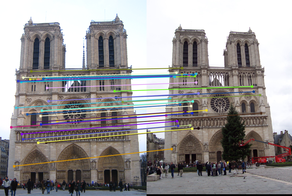
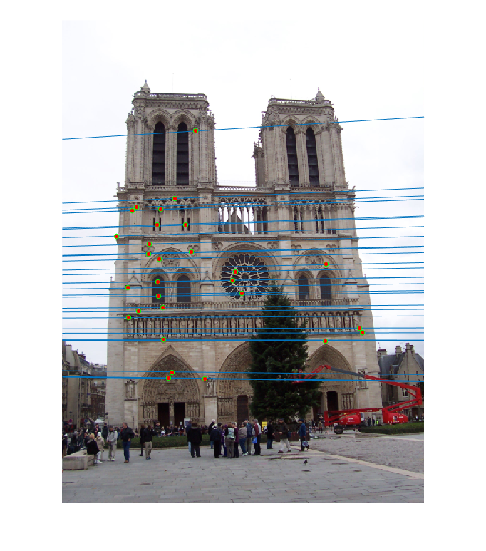
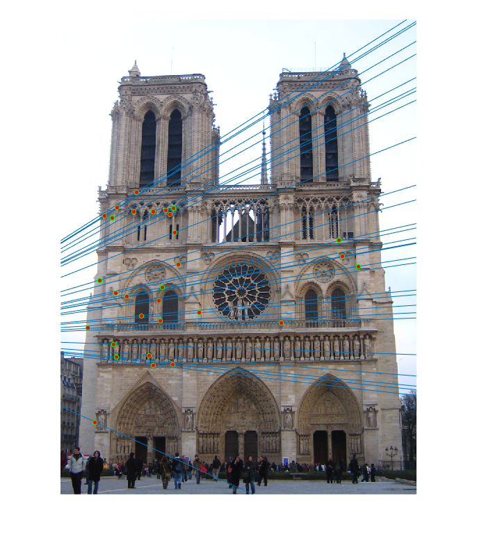
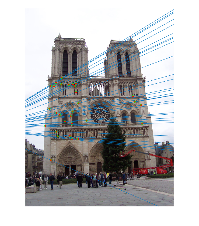
Inlier keypoint correspondences for Notre Dame.
In this project, we estimate the camera projection matrix, which maps 3D world coordinates to image coordinates, as well as the fundamental matrix, which relates points in one scene to epipolar lines in another. The camera projection matrix and the fundamental matrix can each be estimated using point correspondences. To estimate the projection matrix (camera calibration), the input is corresponding 3d and 2d points. To estimate the fundamental matrix the input is corresponding 2d points across two images. This project consists of following parts.
- Part I: Camera Projection Matrix
- Part II: Fundamental Matrix Estimation
- Part III: Fundamental Matrix with RANSAC
- Part IV: Graduate Credit Work - Coordinate Normalization
- Part V: Extra - Extra Credit Work - Parameter Tuning
Part I: Camera Projection Matrix
Fig.1: Homogeneous linear system to find projection matrix M.
The goal is to compute the projection matrix that goes from world 3D coordinates to 2D image coordinates. Recall that using homogeneous coordinates the equation for moving from 3D world to 2D camera coordinates is as in Figure-1.
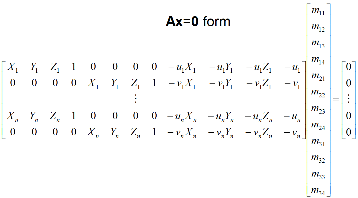
Fig.2: Homogeneous linear system in Ax=0 form.
Another way of writing this equation as in Figure-2. At this point, we are ready to solve this equation for projection matrix M's entries by using linear least squares. We use the singular value decomposition to directly solve the constrained optimization problem:
min||Ax||, s.t. ||x||=1
We use svd() function provided by Matlab to find M matrix as presented in following code block that resides in calculate_projection_matrix.m function.
function M = calculate_projection_matrix( Points_2D, Points_3D )
nPoints=size(Points_2D,1);
A=zeros(nPoints*2,12);% Create the Matrix A where in Ax=0.

% Assign A matrix values with respect to Ax=0 form.
A(1:2:end,1:4)=[Points_3D ones(nPoints,1)];
A(2:2:end,5:8)=[Points_3D ones(nPoints,1)];

A(1:2:end,9:12) =-1.*[repmat(Points_2D(:,1),1,3).*Points_3D Points_2D(:,1)];
A(2:2:end,9:12) =-1.*[repmat(Points_2D(:,2),1,3).*Points_3D Points_2D(:,2)];

[~,~,V]=svd(A);% Apply singular value decomposition to matrix A
M = V(:,end);% Reshape projection matrix M.
M = reshape(M,[],3)';
Here is the comparison between random M matrix and solved M matrix according to given 3D world and 2D camera coordinates. While the residual for the random M points is 31.5146, it is 0.0445 for the calculated projection matrix M. Points in randomly assigned and calulated projection matrices are presented in Figure-3 and Figure-4, respectively.
The randomly assigned projection matrix is: 0.1768 0.7018 0.7948 0.4613 0.6750 0.3152 0.1136 0.0480 0.1020 0.1725 0.7244 0.9932 The total residual for random M is: 31.5146 |
The calculated projection matrix is:
   -0.4583    0.2947    0.0140   -0.0040
    0.0509    0.0546    0.5411    0.0524
   -0.1090   -0.1783    0.0443   -0.5968
The total residual for calculated M is: 0.0445
|
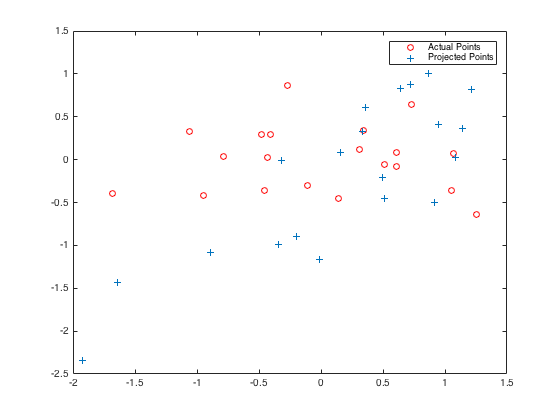
Fig.3: Randomly assigned projection matrix M points. |
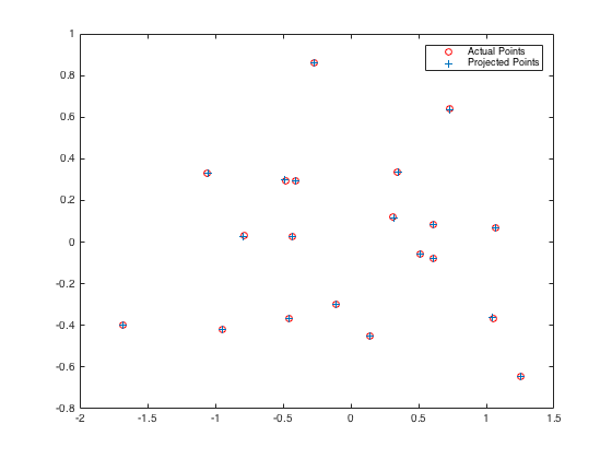
Fig.4: Calculated projection matrix M points. |
Now, we have an accurate projection matrix M, it is possible to tease it apart into the more familiar and more useful matrix K of intrinsic parameters and matrix [R | T] of extrinsic parameters. We only estimate one particular extrinsic parameter: the camera center in world coordinates. Let projection matrix M is defined as M = ( Q|m4 ), where Q is 3x3 matrix and m4 is a column vector. Then, the camera center C could be found by C = - Q-1 m4 equation. The estimated location of camera is ( -1.5127, -2.3517, 0.2826 ). Moreover, Figure-5 shows the estimated camera center with respect to the normalized 3D point coordinates.
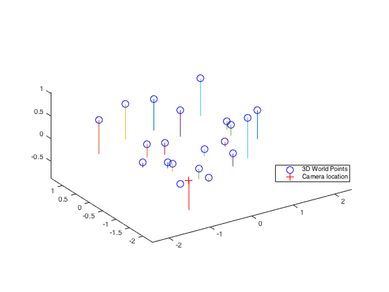
Fig.5: Estimated camera center at (-1.5127, -2.3517, 0.2826) with respect to the normalized 3D point coordinates.
Part II: Fundamental Matrix Estimation
Fig.6: The definition of the fundamental matrix F.
In this part of the project consists of estimating the mapping of points in one image to lines in another by means of the fundamental matrix. This will require to use similar methods to those in part 1. We use the corresponding point locations listed in pts2d-pic_a.txt and pts2d-pic_b.txt. Recall that the definition of the Fundamental Matrix is presented in Figure-6, which gives us following equation in xTFx' = 0 form:
f11uu' + f12vu' + f13u' + f21uv' + f22vv' + f23v' +f21u + f32v + f33 = 0
From above equation, we can create following regression equation in Af = 0 form as presented.
At this point, we are ready to solve this equation for F in full rank by using least squares estimate as in Part-I. Hence, we use the singular value decomposition again to solve this equation.
Since the fundamental matrix is a rank 2 matrix. As such we must reduce its rank. In order to do this we can decompose F using singular value decomposition into the matrices U Σ V' = F.
We can then estimate a rank 2 matrix by setting the smallest singular value in Σ to zero thus generating Σ2 . The fundamental matrix is then easily calculated as F = U Σ2 V'.
We use svd() function provided by Matlab to find f and F matrices as presented in following code block that resides in estimate_fundamental_matrix.m function.
function [ F_matrix ] = estimate_fundamental_matrix(Points_a,Points_b)
xa=Points_a(:,1);
ya=Points_a(:,2);

xb=Points_b(:,1);
yb=Points_b(:,2);

A = [ xb.*xa xb.*ya xb yb.*xa yb.*ya yb xa ya ones(size(xa))];
[~,~,V] = svd(A,0);
f = V(:,end);
F = reshape( f,[3 3])';

[U,S,V] = svd(F);
S(3,3) = 0;
S = S / S(1,1);
F = U * S * V';
Figure-7 and Figure-8 show the epipolar lines for both fundamental matrices in full rank-Ff and in rank two-F2, which are presented below, respectively.
Fundamental Matrix in full rank. -0.000000660698417 0.000007910316208 -0.001886001976909 0.000008823962961 0.000001213829330 0.017233290107265 -0.000907382302153 -0.026423464990181 0.999500091906723 |
Fundamental Matrix in rank 2 matrix. -0.000000536264198 0.000007903647709 -0.001886002040236 0.000008835391841 0.000001213216850 0.017233290101449 -0.000907382264408 -0.026423464992203 0.999500091906703 |

|

|
|
Fig.7: Epipolar lines for the fundamental matrix Ff in full rank. |
|
|
|
|
Fig.8: Epipolar lines for the fundamental matrix F2 in rank 2 matrix. |
|
Part III: Fundamental Matrix with RANSAC
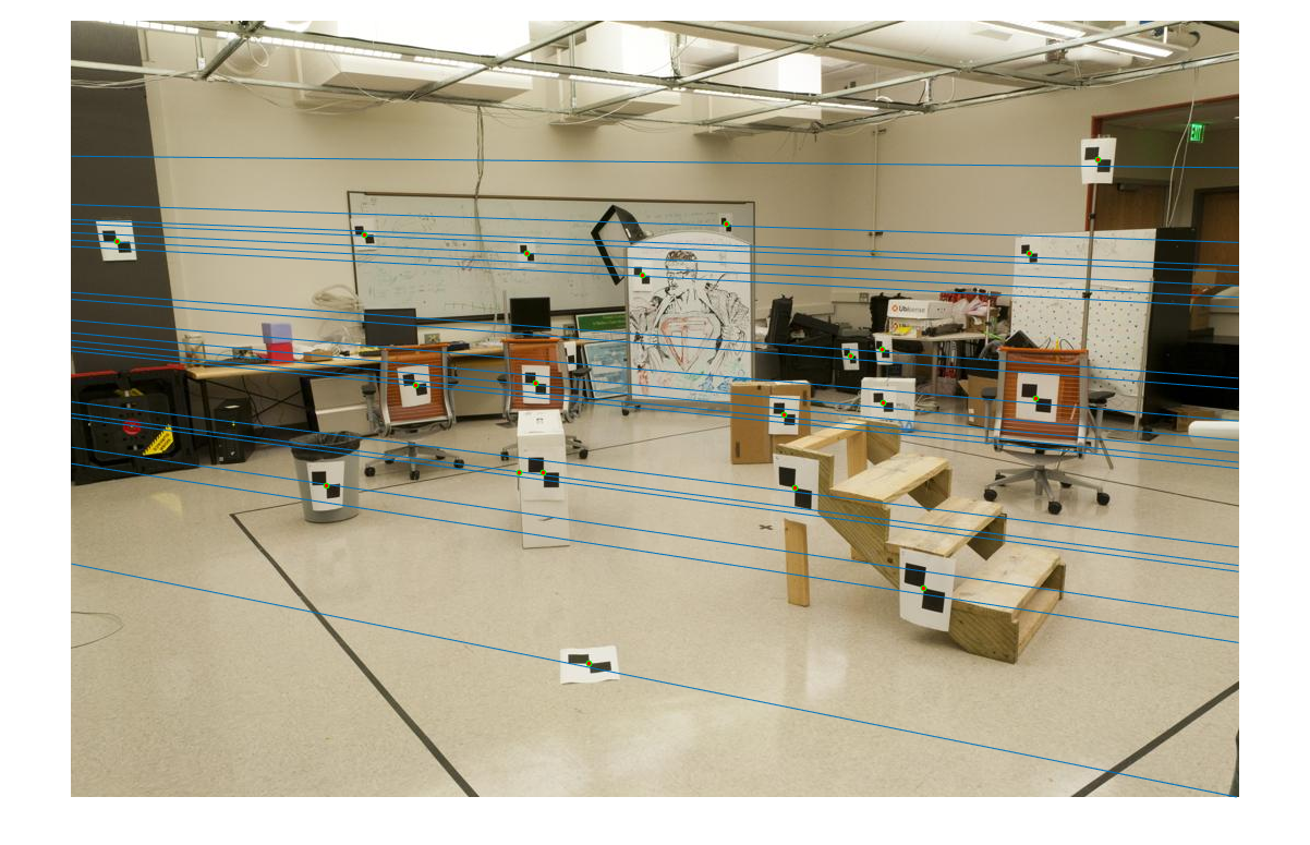
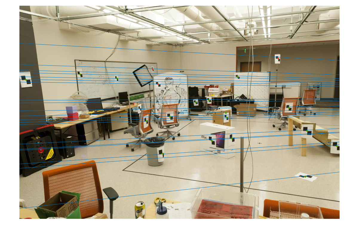
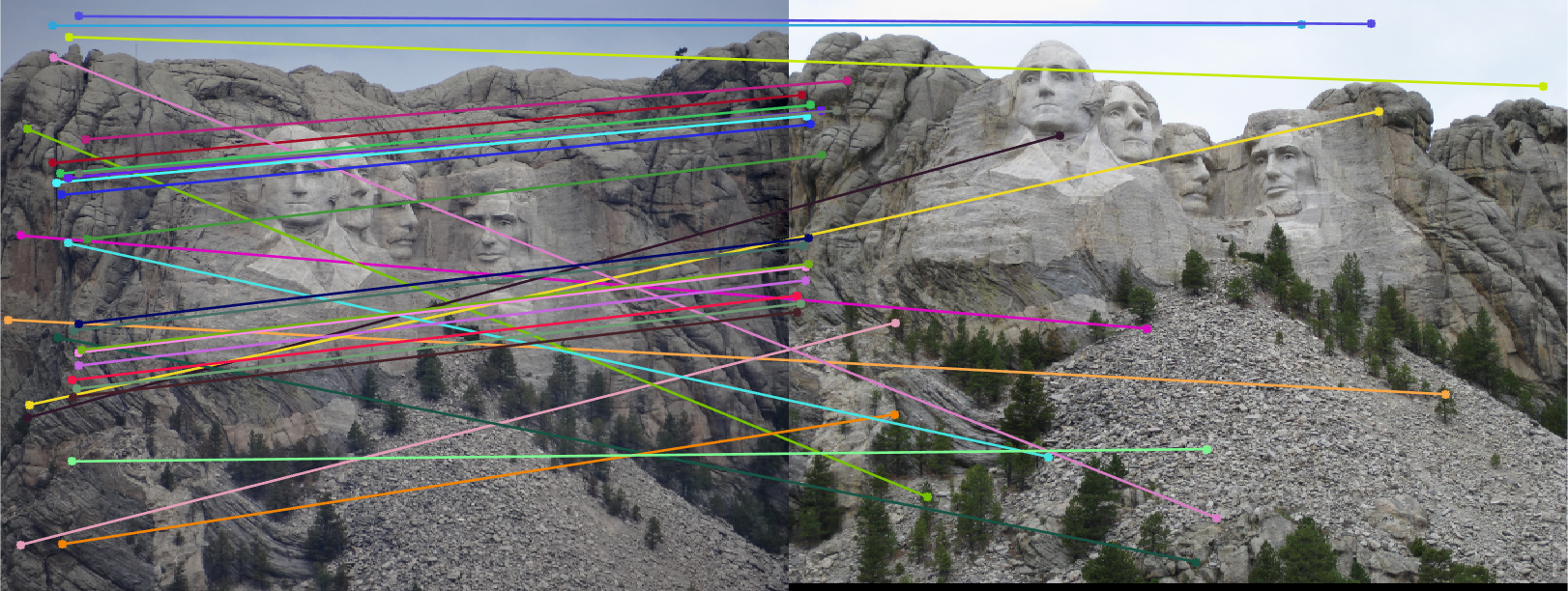
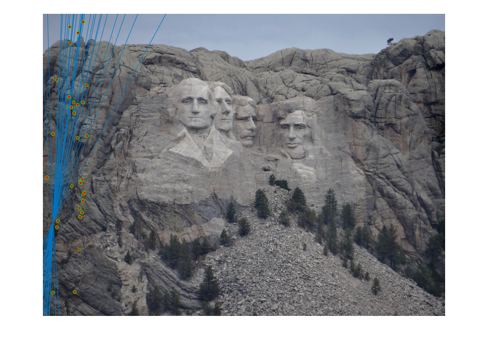
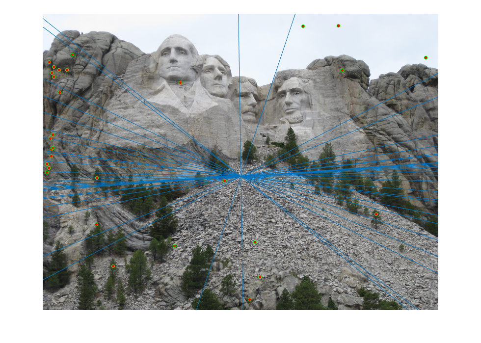
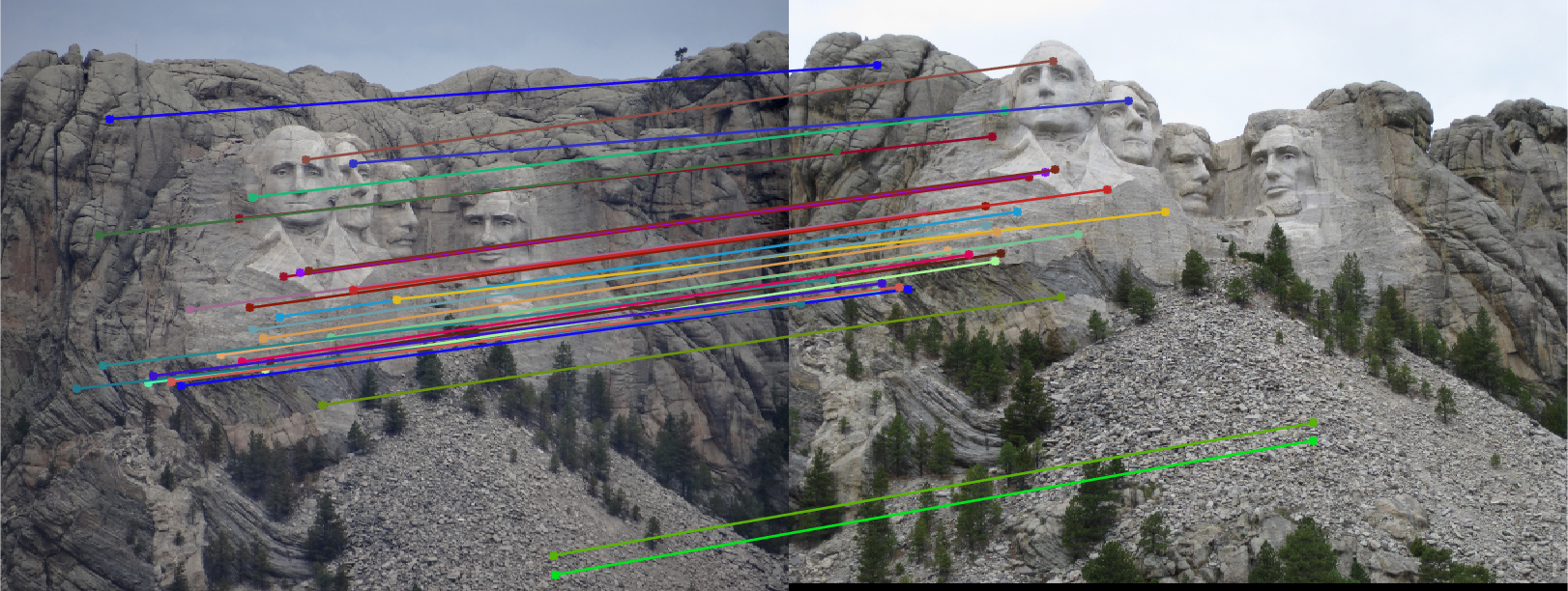
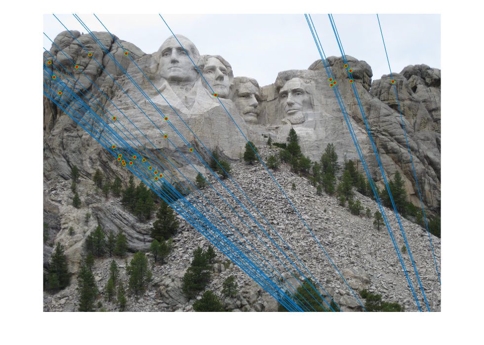
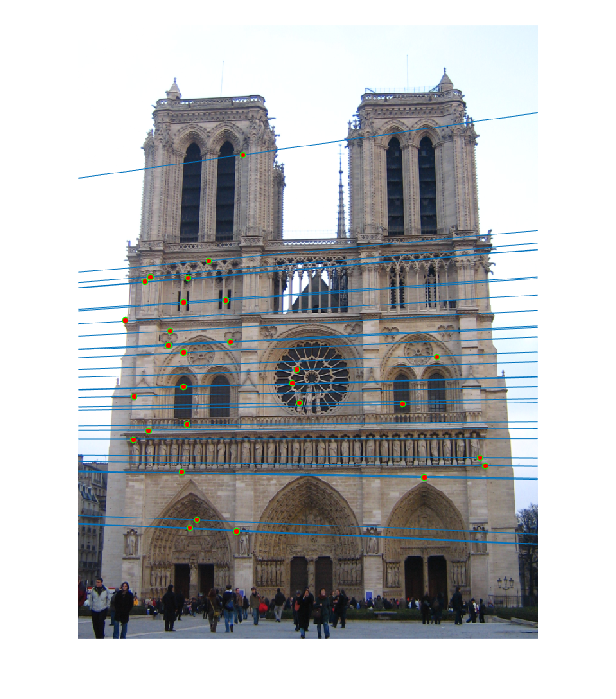
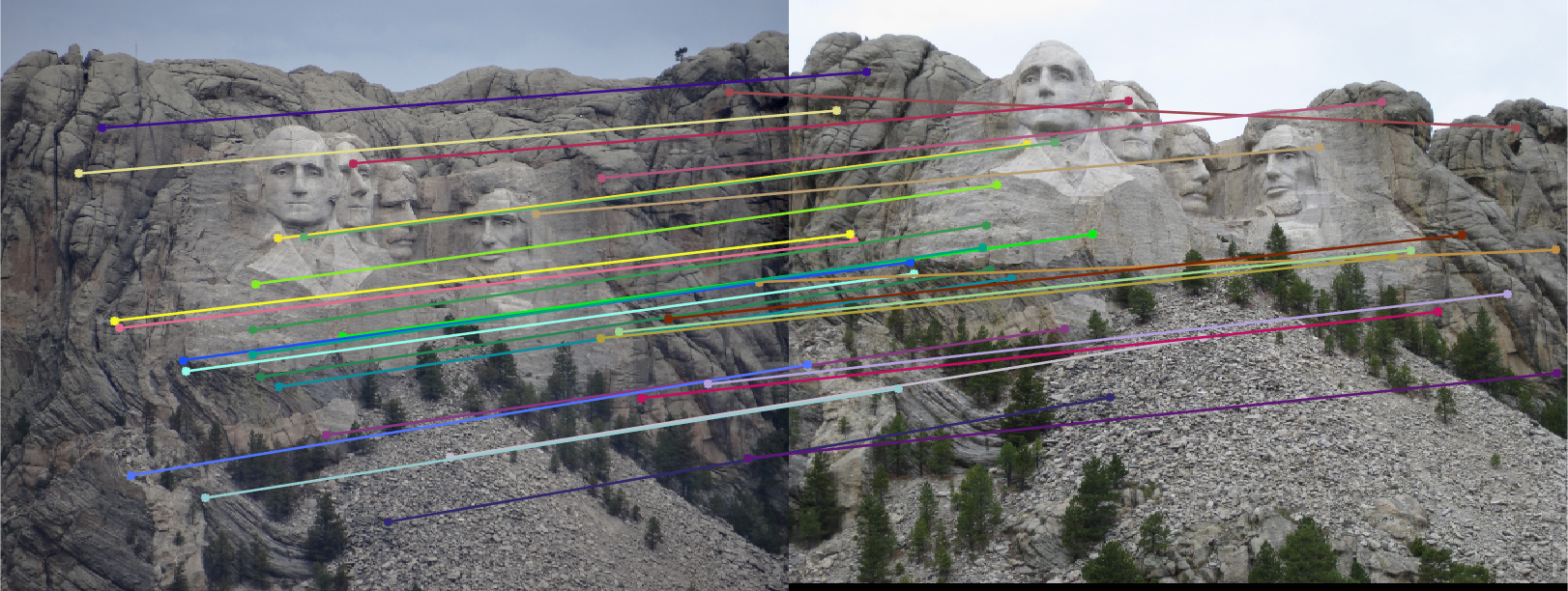
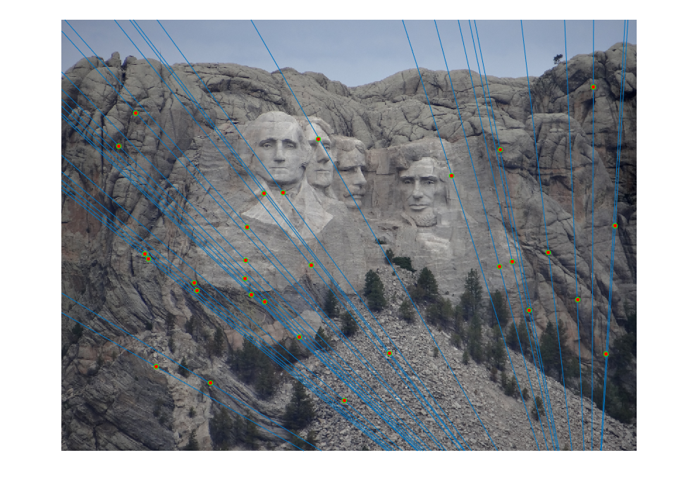
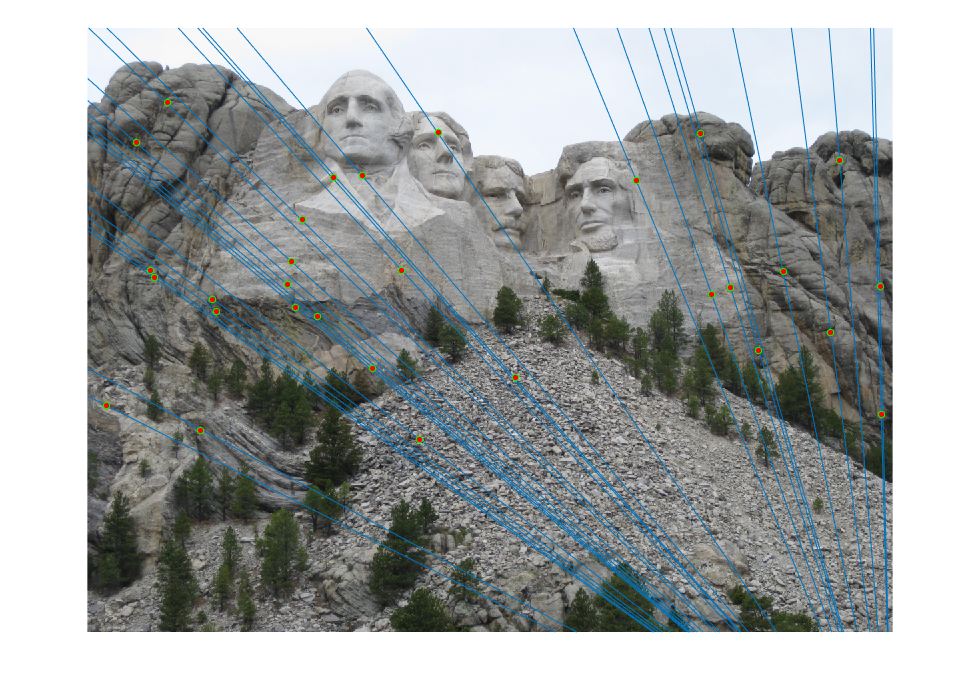
In this part, we compute the fundamental matrix with unreliable point correspondences computed with SIFT. Least squares regression is not appropriate in this scenario due to the presence of multiple outliers. In the following figures, we present all and 30 best SIFT feature matches, and, epipolar lines corresponding fundamental matrix which calculated with 10 best matches in case of not using RANSAC for fundamental matrix estimation. As we see from the figures, in order to estimate the fundamental matrix from this noisy data we need to use RANSAC in conjunction with the fundamental matrix estimation.

|
|
|
Fig.9: All and 30 best SIFT matches without RANSAC for Mount Rushmore image pair. |
|
|
|
|
Fig.10: Epipolar lines for the fundamental matrix F estimated without RANSAC for Mount Rushmore image pair. |
|
At this point, we use these putative point correspondences and RANSAC to find the "best" fundamental matrix. For this, we iteratively choose some number of point correspondences (s=8 for this case), solve for the fundamental matrix using the function in Part II, and then count the number of inliers. Inliers in this context are point correspondences that "agree" with the estimated fundamental matrix. In order to count how many inliers a fundamental matrix has, we use a distance metric (dT=1.5 for this case) based on the fundamental matrix. Recall that for a point correspondence (x',x) we have xTFx'=0 property. Hence, if this property close enough to zero (say < 0.01 for this case), we count this point correspondence (x',x) as inlier. Moreover, we need to pick a threshold between inlier and outlier. Since our results are very sensitive to this threshold, we need to explore a range of values. Thus, we pick p=0.99 and e=0.1, which are confidence and outlier rejection rate, respectively, to define this threshold. After N trials, we return the fundamental matrix with the most inliers. The number of N is determined as follows:
N= log( 1-p ) / log( 1-(1-e)s)
The physical meaning of N is that the number of iterations we can achive p=0.99 confidence for inliers. Following code block presents the RANSAC algorithm that resides in ransac_fundamental_matrix.m function.
function [ Best_Fmatrix, inliers_a, inliers_b] = ransac_fundamental_matrix(matches_a, matches_b)
matches_a(:,3)=1;
matches_b(:,3)=1;
% Set free parameters
e=.1;
p=.99;
s=8;
N=log(1 - p)/log(1 - (1 - e)^s);
cnt=0;
maxInliers=0;
bestDistErr = Inf;
dT=1.5;

while cnt < N
    rs=randsample(size(matches_a,1),8);
    r8_match_a=matches_a(rs,1:2);
    r8_match_b=matches_b(rs,1:2);
    cnt=cnt+1;

    % Call fundamental matrix calculation from Part-II.
    F=estimate_fundamental_matrix(r8_match_a,r8_match_b);

    % Find inliers from correspondence points.
    L1=normLine(F*matches_a');
    d1=abs(dot(matches_b',L1));

    L2=normLine(F'*matches_b');
    d2=abs(dot(L2,matches_a'));

    inliers = find( d1 < dT & d2 < dT );
    inlierCount = size(inliers,2);

    % Check and update overall distance error for inliers.
    if inlierCount > 0
        distErr = sum( d1(inliers).^2 + d2(inliers).^2 ) / inlierCount;
    else
        distErr = Inf;
    end
    % Check and update best fundamental matrix and corresponding inliers and distance error.
    if inlierCount > maxInliers || (inlierCount == maxInliers && distErr < bestDistErr)
        maxInliers = inlierCount;
        bestDistErr = distErr;
        Best_Fmatrix = F;
        bestInliers = inliers;
    end

end

% randomly pick 30 inliers
samples=randsample(numel(bestInliers),30);
inliers_a = matches_a(bestInliers(samples),1:2);
inliers_b = matches_b(bestInliers(samples),1:2);
end

function Lnorm=normLine(L)
Lnorm=L./repmat(sqrt( L(1,:).^2 +L(2,:).^2 ),3,1);
end
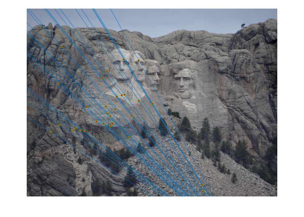
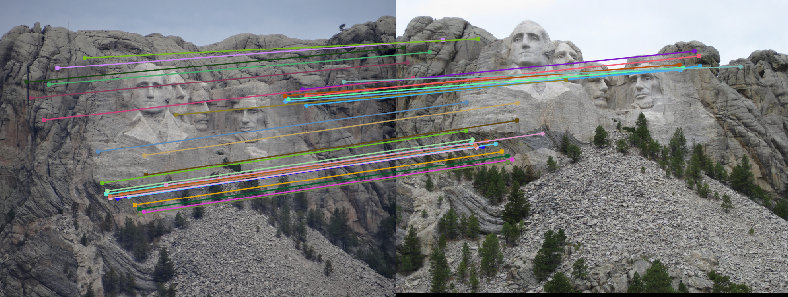
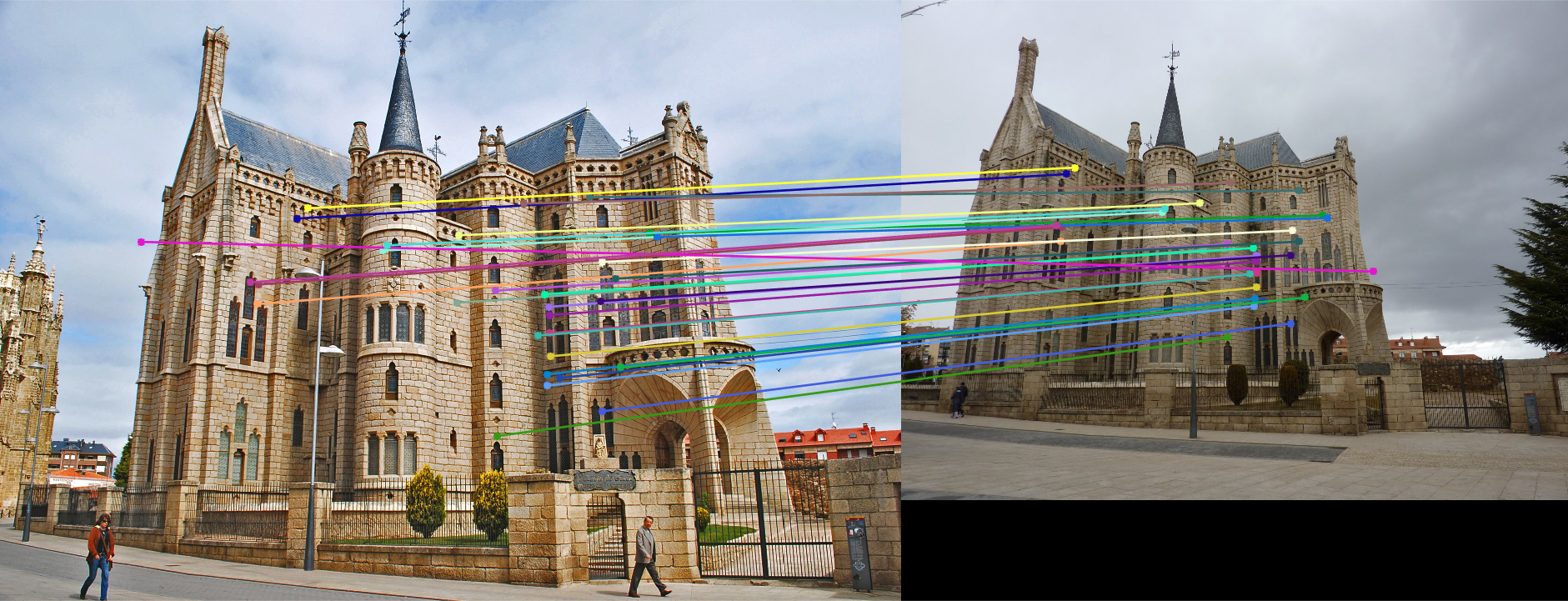
After applying RANSAC, we found following best fundamental matrix with overall distance error of 1.3098. Also, we present the 30 inlier point matches and epipolar lines for this fundamental matrix in Figure-11 and Figure-12, respectively.
Note: It is worth to note that there is no normalization adapted in fundamental matrix estimation in Part-II yet. Their results will be presented following Extra Credit section.
Fundamental Matrix used in Fig.10 without using RANSAC.
   -0.0000   -0.0000    0.0004
   -0.0000   -0.0000    0.0015
    0.0088    0.0011   -1.0000
|
Fundamental Matrix used in Fig.12 by using RANSAC. Overall distErr=1.3098
   -0.0000    0.0000   -0.0382
   -0.0000   -0.0000    0.0386
    0.0380   -0.0346    0.9972
|
|
|
|
|
Fig.11: Putative 30 best SIFT matches without RANSAC (Fig.9(right)) and 30 inliers correspondence matches for Mount Rushmore image pair. |
|
|

|
|
Fig.12: Epipolar lines for the best fundamental matrix estimated by using RANSAC for Mount Rushmore image pair. |
|
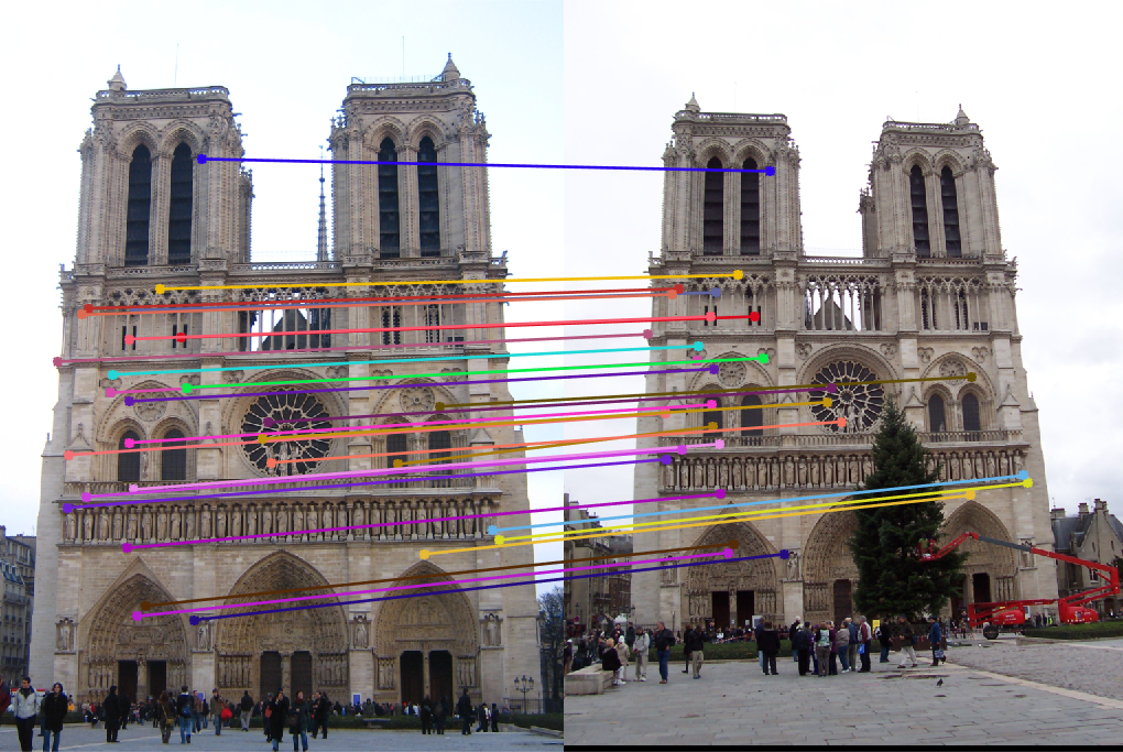
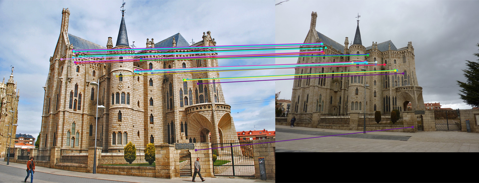
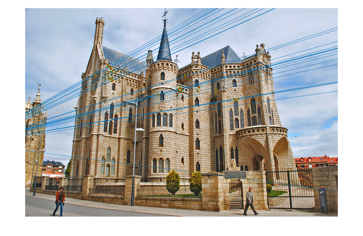
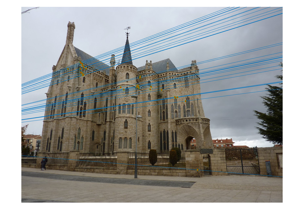
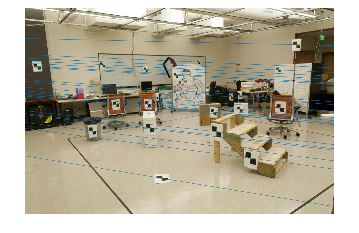
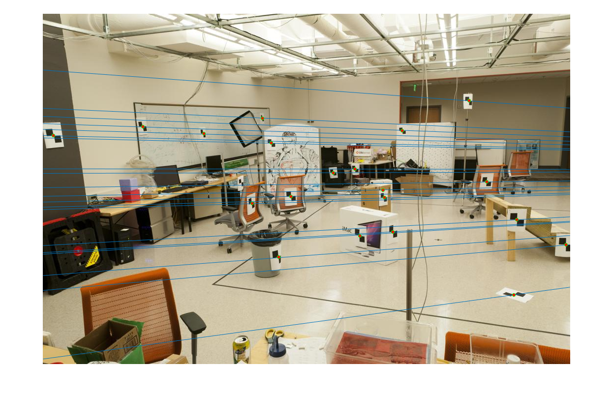
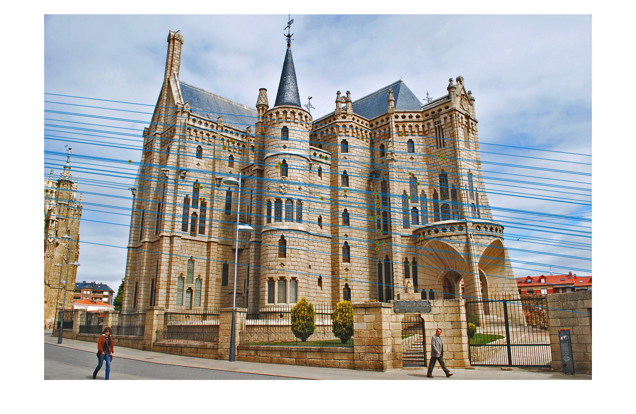
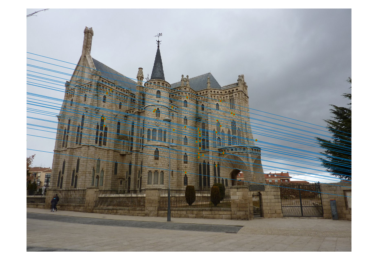
In the following figures, we present several different images with the epipolar lines drawn on them and with the inlier keypoint correspondences shown. Calculated best fundamental matrices and corresponding overall distance errors are also presented for each images. It is worth to note that we have to set e=0.3 to get enough inliers for Figure-15.
|
|
|
|||

|
|
|
|
|
|
|
Fig.13: Mount Rushmore. |
Fig.14: Notre Dame. |
Fig.15: Episcopal Gaudi. |
|||
Overall distance error = 1.8046. -0.0000 0.0000 -0.0390 -0.0000 -0.0000 0.0360 0.0387 -0.0327 0.9973 |
Overall distance error = 0.8712. -0.0000 0.0000 -0.0026 -0.0000 0.0000 -0.0278 0.0055 0.0231 0.9993 |
Overall distance error = 1.3776. 0.0000 -0.0000 0.0255 0.0000 -0.0000 0.0282 -0.0275 -0.0121 0.9988 |
|||
Part IV: Graduate Credit Work - Coordinate Normalization
In this part, we perform normalization to the coordinates to improve fundamental matrix estimation in Part-II. We apply the normalization through linear transformations as described below to make the mean of the points zero and the average magnitude square root of 2. Here is the transform matrix T in form of T = S * O, where S is scale and O is offset matrices. And, the usage of T is in form of C' = T * C as below:
, where s is scale, cu and cv are the mean coordinates in offset O matrix, u and v are coordinates of given key points, and u' and v' are the scaled coordinates. To compute a scale s we estimate the standard deviation after substracting the means from coordinates. And, we calculate scale matrix S for each image. After scaling our coordinates, we apply denormalization to fundamental matrix Fnorm to get original fundamental matrix as:
Forig = T'T * Fnorm * T
Following code blocks present the normalization of coordinates and updated version of estimate_fundamental_matrix.m function.
|
|
We normalize the coordinates listed in pts2d-pic_a.txt and pts2d-pic_b.txt and plot the epipolar lines as presented in Figure-16 and compare it with Figure-8 along with fundamental matrices.
|
|
|
|
|
|
Fig.16: Epipolar lines for the fundamental matrices (Top Images:) from non-normalized coordinates and (Bottom Images:) from normalized coordinates. |
|
F from non-normalized coordinates. Used in Top Images. -0.000000536264198 0.000007903647709 -0.001886002040236 0.000008835391841 0.000001213216850 0.017233290101449 -0.000907382264408 -0.026423464992203 0.999500091906703 |
F from normalized coordinates. Used in Bottom Images. -0.000000219742095 0.000003012409266 -0.000752995136854 0.000002083373401 -0.000000511974656 0.006056268551890 -0.000044060457717 -0.008324532266617 0.193721256393101 |
After updating the fundamental matrix estimation with coordinate normalization, we again present several different images with the epipolar lines drawn on them and with the inlier keypoint correspondences shown in the following figures. Calculated best fundamental matrices and corresponding overall distance errors are also presented for each images.
|
|
|
|||
|
|
|
|
|
|
|
Fig.17: Mount Rushmore. |
Fig.18: Notre Dame. |
Fig.19: Episcopal Gaudi. |
|||
Overall distance error = 0.8599. 0.0000 -0.0000 0.0076 0.0000 0.0000 -0.0077 -0.0075 0.0068 -0.1857 |
Overall distance error = 0.8409. 0.0000 0.0000 -0.0141 -0.0000 -0.0000 -0.0066 0.0136 0.0055 0.6518 |
Overall distance error = 0.7180. 0.0000 -0.0000 0.0014 -0.0000 -0.0000 -0.0045 -0.0004 0.0043 -0.3344 |
|||
Part V: Extra - Extra Credit Work - Parameter Tuning
In this section, some statistical analysis is made to pick free parameters tuned in Part-III for RANSAC algorithm. First, outlier rate of e is tuned. To do this, we measure maximum number of inliers for each value of e. We iterate e by incrementing it 0.05 each time from 0.05 to 0.5. Moreover, we take 100 averages for each iteration of e to normalize found maximum inliers count. At the same time, we measure the average runtime for each iteration of e to find the trade-off between calculation time of the fundamental matrices and resulted inliers. As we can see from the following boxplot of found maximum number of inliers and average running time for each value of outlier rate e, it is better to choose e=0.1 at minimum to get enough inliers (at least 30 for this case) in all iterations of RANSAC algorithm. On the other hand, increasing the e values is not a costly operation until the value of 0.25. After this point, the running time start increasing more obviously.
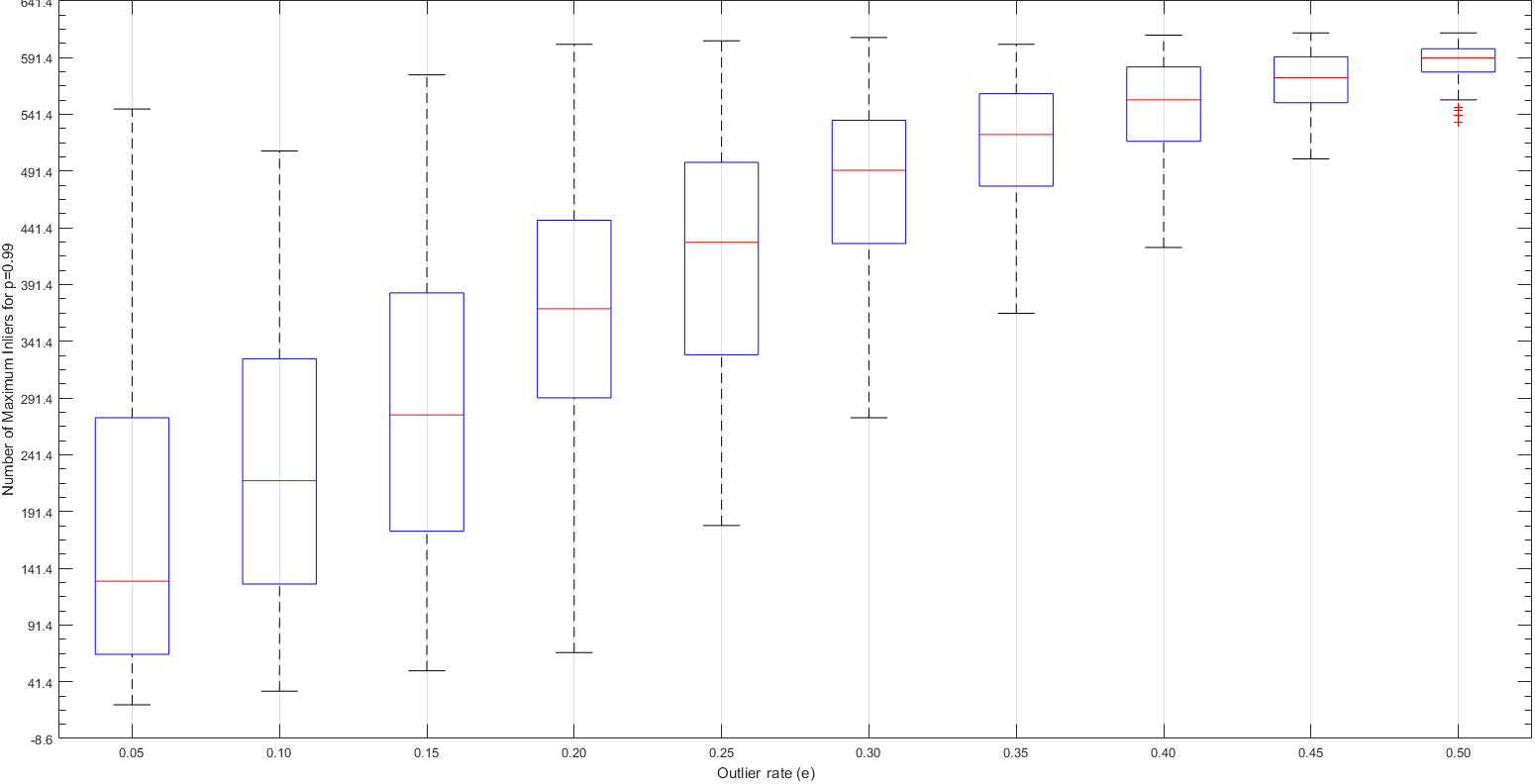
Fig.20: Boxplot of maximum number of inliers for each e values for Mount Rushmore.
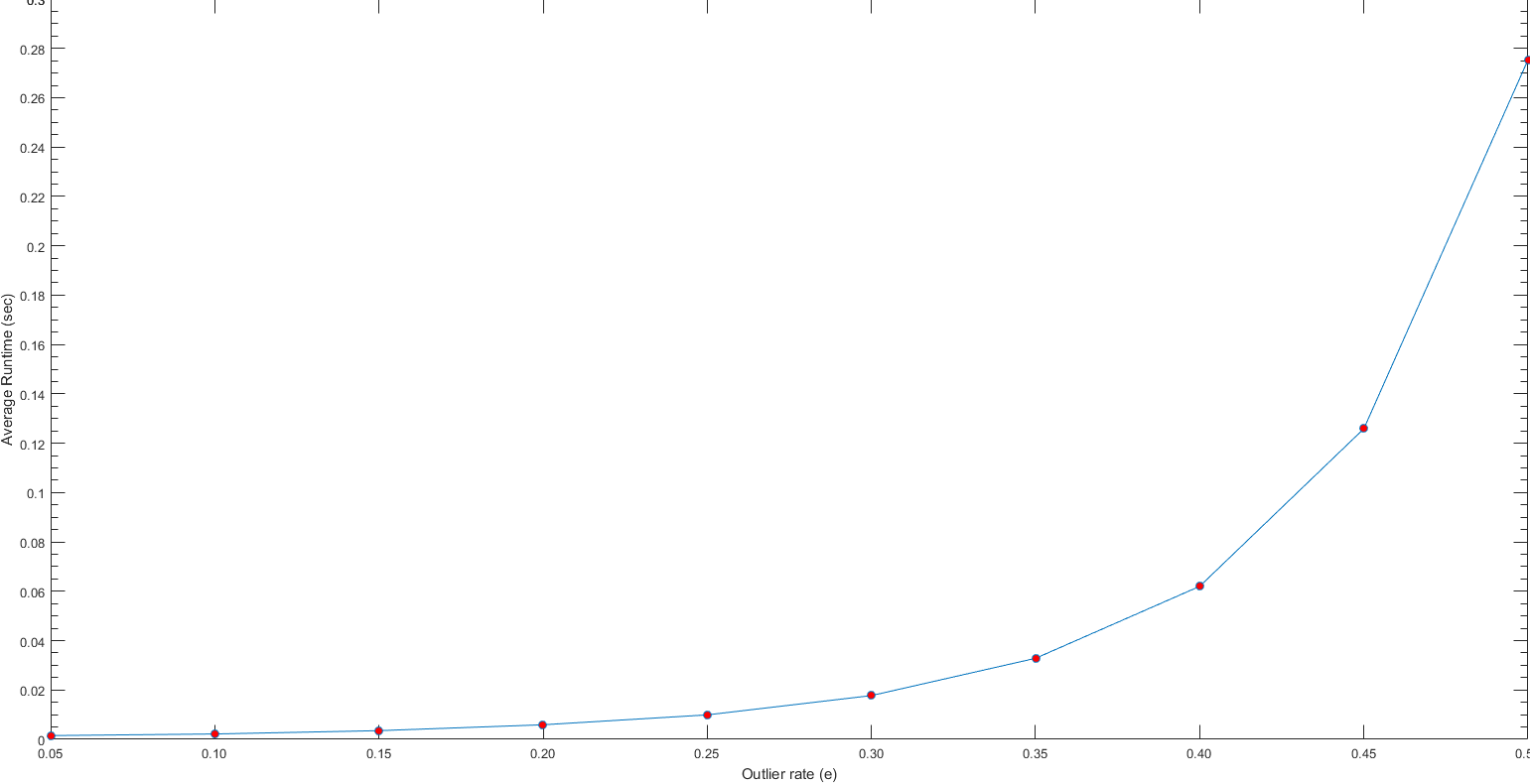
Fig.21: Avera running time for each e values for Mount Rushmore.