Graham Wright

Project 3 / Camera Calibration and Fundamental Matrix Estimation with RANSAC

In this project, our goal is to find ways to map 3D world coordinates to 2D image coordinates as well as relate two different image coordinates with each other. This will allow us to more effectively match points between images that have varying perspectives or scales.

Part 1: M and Camera Center

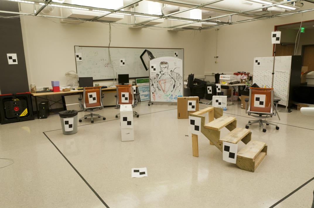
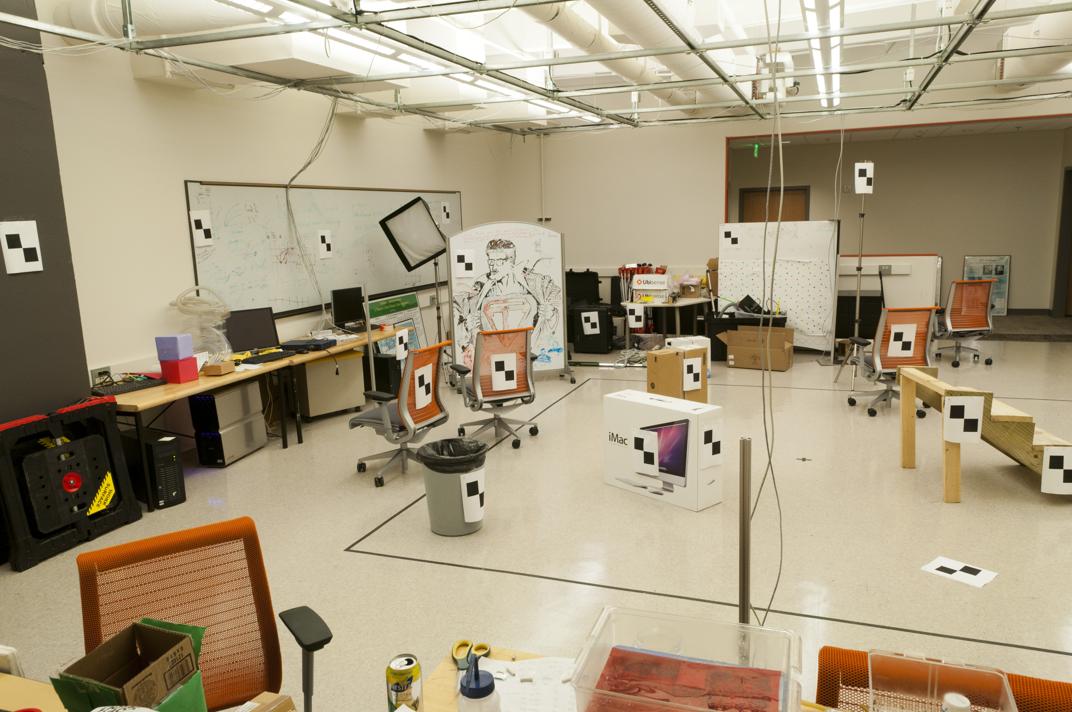
We start with trying to get the projection matrix M that maps 3D world coordinates to 2D image coordinates. We are using known 3D and 2D coordinates from the below images (at the targets) to find the projection matrix.

Some simple linear algebra allows us to retrieve the projection matrix which turns out to be defined up to a scale of -1.

The projection matrix is:

-0.4583	0.2947	0.0140	-0.0040
0.0509	0.0546	0.5411	0.0524
-0.1090	-0.1783	0.0443	-0.5968

The total residual is 0.0445.

We can then perform some singular value decomposition to recover the camera center in the 3D space:

The estimated location of camera is: <-1.5127, -2.3517, 0.2826>

Part 2: Fundamental Matrix Unnormalized

Part 2 concerns itself with finding the fundamental matrix that relates coordinates between image pairs. We use 8+ point pairs to solve for the fundamental matrix with the 8 point algorithm. We also reduce the rank of the matrix we find so that we end up with a rank 2 matrix. One method of improving this matrix discovery is to normalize points before running the algorithm. This first part does not normalize the points.

F_matrix =

-0.0000	-0.0000	-0.0019
0.0000	0.0000	0.0172
-0.0009	-0.0264	0.9995

Here are the corresponding epipolar lines between the images in the pair:

Without reducing the rank of the matrix, we get epipolar lines that travel straight through the points. However, after reducing the rank, some lines tend to clip the bottom or tops of the points. This is most likely a result of slight imprecision in coordinate measurements.

Part 2: Fundamental Matrix Normalized

This time around, we normalize the coordinate points before solving for the fundamental matrix. We fix the average of the points at the origin and make the final points an average distance of the square root of 2 from the origin.

F_matrix =

-0.0000	-0.0000	-0.0001
0.0000	-0.0000	0.0008
-0.0000	-0.0010	0.0244

Notice that the epipolar lines travel directly through the middle of the points, showing the positive effects of the normalization.

Part 3: Real Images Unnormalized and Normalized

Now it is time to apply our fundamental matrix computations to more image pairs. First, we use SIFT to gather a set of matching points between the images. Next, we implement RANSAC to iteratively solve for the fundamental matrix with a subset of 8 random points and determine the number of inlying points. We keep track of the matrix that has the most inliers and use that for our correspondence between the images. We will alternate between unnormalized and normalized fundamental matrix solving methods to see if there is any noticeable performance boost from normalization.

d is the distance threshold. The fundamental matrix relationship tells us that we should get a norm of 0 if we multiply our 2nd image coordinate with our fundamental matrix and the transpose of our 1st image coordinate. We consider a pair of points to be an inlier if the resulting norm is less than our distance threshold.

(Image 1) 5000 iterations, d = 0.001, 78/825 inliers, no norm

(Image 2) 5000 iterations, d = 0.001, 78/825 inliers, no norm Above we have some examples of the epipolar lines projected across the images. As you can see, the lines seem to do a good job of lining up with the points.

(Matching Images) 5000 iterations, d = 0.001, 78/825 inliers, no norm Our image above appears to match very well. Although it is hard to tell from just looking at it, it appears that most if not all points are correctly matched. The only obviously incorrect match I can make out is the brown-orange point that is located under the pink point in the left image.

5000 iterations, d = 0.01, 221/825 inliers, no norm Our distance threshold in the previous image allowed a moderate number of inliers (78). What happens if we loosen the threshold? We get almost 3x the inliers. We seem to still get very consistent matches even with so many inliers. It is difficult to make out any obviously incorrect matches.

5000 iterations, d = 0.0001, 129/825 inliers, normalized One noticeable impact of coordinate normalization is the need for a lower distance threshold to get a similar number of inliers compared to the non-normalized version. As is expected, our normalized version also performs quite well with no obvious mistakes.

1000 iterations, d = 0.01, 666/825 inliers, normalized, 30 randomly sampled So far, we have used fairly high iterations and low distance thresholds. Above, we have loosened both of these parameters and sampled 30 random matches. Notice that we get a whopping 666 inliers - much more than before. A higher distance threshold allows us to find a solution that covers more points which should in theory get us a solution that is closer to the actual solution. Our epipolar lines (not shown) look almost the same as our previous normalized result. It is possible that at a certain number of inliers, extra inliers do not aid our solution. Perhaps filtering out with our distance threshold does not have to negatively affect our final fundamental matrix.

5000 iterations, d = 0.001, 44/851 inliers, no norm Moving to the Notre Dame image, we get a highly accurate correspondence between the two images. This distance threshold limits us to having 44 top inliers which could in some cases negatively affect our results. We have to be careful with our distance threshold since we might reject some true matches just due to imprecision (solving for the fundamental matrix has some ideal assumptions such as the makeup of the cameras). This gets us great results, but we could surely get even more matches.

5000 iterations, d = 0.005, 166/851 inliers, no norm Here we upped the distance threshold, so we got a solution with many more inliers. From skimming the image, I counted only 1 clearly incorrect match! It appears that we have gotten an even better solution with our increased distance threshold.

5000 iterations, d = 0.0001, 67/851 inliers, normalized It appears that we have managed to get 67 solid matches. It would appear that they are all accurate. From results so far, it would seem that 5000 iterations is enough for finding an excellent solution. In theory, increased iterations should give us better fundamental matrices since we have more opportunity to find an optimal matrix. Another interesting point is the drastically different pattern of the epipolar lines. Clearly, RANSAC is so focused on getting inliers that the orientation of the epipolar lines can greatly vary between RANSAC runs with the same parameters. If our algorithm finds inliers that are all in a certain orientation or area, we can see our epipolar projections overfitting.

3000 iterations, d = 0.01, 670/851 inliers, normalized, 30 randomly sampled We again try lowering the iterations and distance threshold. Our sampled 30 points look quite accurate. Most noticeably, our epipolar lines have changed from our last normalized example. Being able to include more inliers appears to have given us a better fundamental matrix. We also get matches that are more spread out. When we limit ourselved to less inliers, these often end up in certain image patches due to the overfitting of the fundamental matrix estimate. With more inliers such as in this example, we can cover the entire range of the image, and our sampling reflects that.

8000 iterations, d = 0.001, 59/616 inliers, no norm Our image of Woodruff gives us great results with these parameters. However, it is interesting to note that sometimes we get some wacky matches with this configuration. It seems that increasing the number of iterations helps this, as is expected.

8000 iterations, d = 0.0001, 69/851 inliers, normalized Our normalized version with 69 inliers does not seem to have any obvious mismatches. Interestingly, we see what appears to be a more accurate estimation of the fundamental matrix as seen in the epipolar line projections. Again, this appears to be a result of our distance threshold. It would appear that the normalization allows us to solve for a better fundamental matrix while needing fewer inliers (as chosen by our distance threshold).

3000 iterations, d = 0.01, 221/851 inliers, normalized, 30 randomly sampled Loosening our parameters, we end up with at least 2 incorrect matches in our randomly chosen 30 inliers. Our fundamental matrix looks very similar to our last normalized example, so there is not much else to report in that respect.

8000 iterations, d = 0.001, 92/1062 inliers, no norm The Gaudi image is the real test. With our non-normalized run, we end up getting moderate accuracy. Many points match incorrectly across the image or into the sidewalk. However, there are patches of the image that do very well. Here, we increased our iterations to 8000 as we know this is a more difficult pair.

8000 iterations, d = 0.0001, 59/1062 inliers, normalized Our nomalized version (with a few more iterations) performs even better. From skimming the image, I don't see any obvious mismatches, giving us a much higher accuracy than the non-normalized version. It was not clear with our easier images if coordinate normalization actually improved matching performance, but this image pair is a great showcase of the possible improvements. The epipolar lines also make more sense than the non-normalized version. This normalized run managed to attract inliers that span across the whole image rather than just images at certain clusters of the image. This allowed for a better display of epipolar lines.

3000 iterations, d = 0.01, 498/1062 inliers, normalized, 30 randomly sampled Our sampled version with looser paremeters also performs quite well. Our epipolar lines are similar to our last normalized example, except this time slightly more converging off the images. There is at least one incorrect match (mid shade blue, maybe red), but overall, the matches are very good as well.

Conclusion

Solving for the fundamental matrix with RANSAC after performing SIFT matching appears to be quite effective in matching 2 image interest points. There is certainly some variation in effectiveness among the image pairs which are not necessarily obvious. Fortunately, our methodology seems to be fairly effective even without much tweaking. Image pairs similar to our Gaudi example benefit greatly from coordinate normalization. It seems that normalization is not required for simpler image pairs. With parameter tweaking (iterations and distance threshold), however, we really optimize our accuracy within image pairs. Often, finding our fundamental matrix with RANSAC gives us a matrix that can properly match image points even though it might not be the closest in orientation to the real fundamental matrix. There are sometimes multiple matrices that will produce the best number of inliers depending on the distance threshold and RANSAC iterations. If we are just trying to get some matching image points, this isn't that important, but in theory, it might take some eipolar visualization to get a feel for which one is actually more correct. Another effective method is to loosen the distance threshold so that we end up with many outliers. The more chance for more inliers, the more points RANSAC can agree with in the end. This might be the key to getting the best estimate of the fundamental matrix.