Project 3 / Camera Calibration and Fundamental Matrix Estimation with RANSAC
Overview
For this project, pairs of images of the same scene were used for camera calibration and estimation of the fundamental matrix. In the first part of the project, the camera center was recovered by computing the projection matrix given a mapping of 3D to 2D points and their correspondences to the same points in another image. For the second part, the epipolar lines for the same two images were computed by estimating the fundamental matrix given the point mapping. The third part of this project then used this estimation in combination with RANSAC to identify the most confident interest point matches and their epipolar lines for images without a known mapping.
Part I
 |
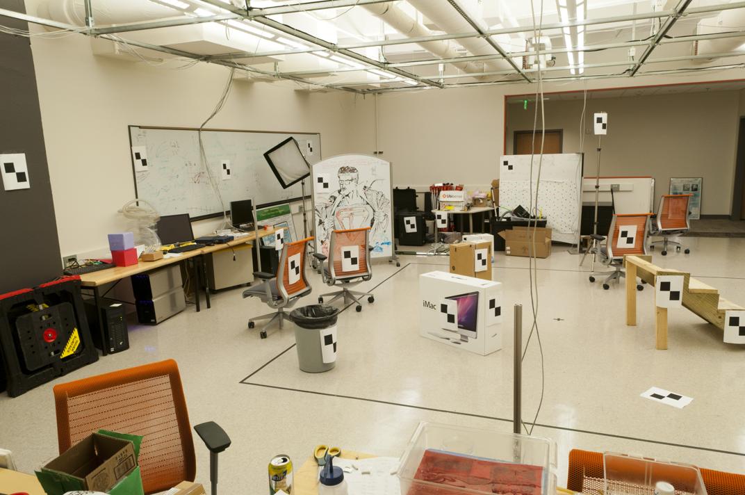 |
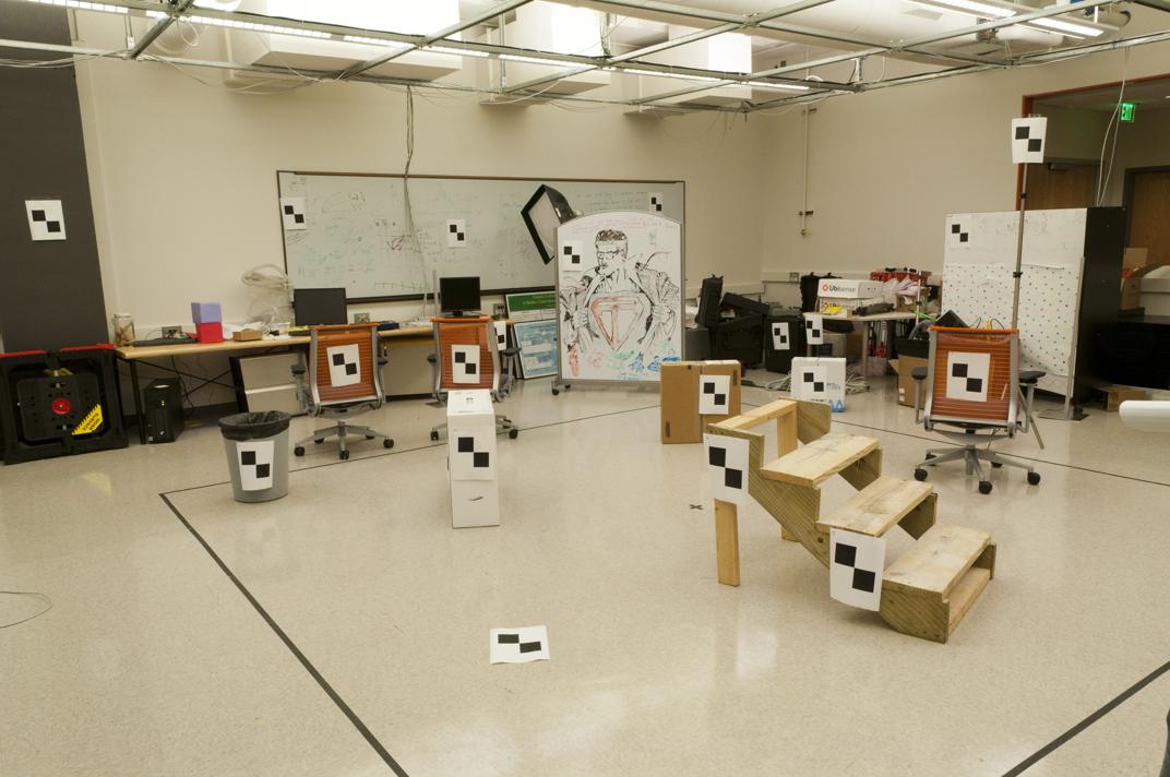
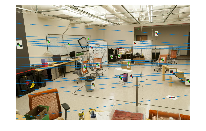
Part I of the project involved calibrating the camera using a pair of images (above) with point correspondences. To do this, the first step was to calculate the projection matrix given these correspondences. This was implemented in the Matlab calculate_projection_matrix() function shown below:
% Get A matrix
uv = Points_2D';
uv = uv(:);
xyz = zeros(length(uv), 11);
for i = 1:2:length(uv)
    pt3 = Points_3D(floor(i/2)+1,:);
    pt2 = Points_2D(floor(i/2)+1,:);
    xyz(i:i+1,:) = [pt3, 1, zeros(1,4), -pt2(1)*pt3;
                    zeros(1,4), pt3, 1, -pt2(2)*pt3];
end

% Use SVD to solve for M matrix
[~, ~, V] = svd([xyz, -uv]);
M = reshape(V(:,end),[],3)';
This code sets up the system of equations AM = Y, where M is the desired projection matrix, Y is the set of 2D point correspondences, and A is the matrix establishing the system of equations relating the projection matrix to the 2D points. SVD is then used to solve this system of equations to recover the M matrix. The projection matrix estimated using this function and the residual error is shown below:
The projection matrix is:
    0.4583   -0.2947   -0.0140    0.0040
   -0.0509   -0.0546   -0.5411   -0.0524
    0.1090    0.1783   -0.0443    0.5968


The total residual is: <0.0445>
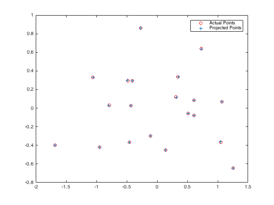
As shown above, the residual for the projection matrix is very small, and the projected points lie very close to the actual points.
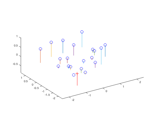
After computing the projection matrix, this matrix can be used to determine an estimate of the camera center using the code below in the Matlab function compute_camera_center():
% Find camera center from M matrix (C = -Q^(-1) * m4)
Q = M(:,1:3);
m4 = M(:,4);
Center = -Q\m4;
The resulting estimate for the camera center is as follows:
The estimated location of camera is: <-1.5127, -2.3517, 0.2826>
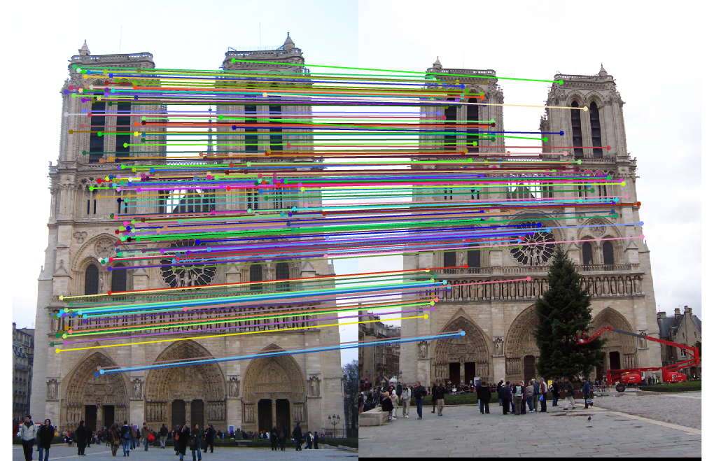
Part II
For the second part of this project, the fundamental matrix was estimated for the same image pair as Part I. Additionally, the point correspondences were normalized to avoid poor numerical conditioning for points near the edges of the image. This was implemented in the estimate_fundamental_matrix() function in Matlab:
u = Points_a(:,1);
v = Points_a(:,2);
u_prime = Points_b(:,1);
v_prime = Points_b(:,2);

% Get mean and std for normalization
umean = mean([u; u_prime]);
vmean = mean([v; v_prime]);
ustd = 1/std([u - umean; u_prime - umean]);
vstd = 1/std([v - vmean; v_prime - vmean]);

% Get normalization matrix
T = [ustd, 0, 0; 0, vstd, 0; 0, 0, 1] * [1, 0, -umean; 0, 1, -vmean; 0, 0, 1];

% Transform points
u = ustd * (u - umean);
v = vstd * (v - vmean);
u_prime = ustd * (u_prime - umean);
v_prime = vstd * (v_prime - vmean);

% Get A matrix
A = zeros(size(Points_a,1),9);
A(:,1) = u .* u_prime;
A(:,2) = v .* u_prime;
A(:,3) = u_prime;
A(:,4) = u .* v_prime;
A(:,5) = v .* v_prime;
A(:,6) = v_prime;
A(:,7) = u;
A(:,8) = v;
A(:,9) = ones(size(Points_a,1),1);

% Get F_matrix with SVD
[~, ~, V] = svd(A);
f = V(:,end);
F_matrix = reshape(f, [3, 3])';

% Enforce singularity
[U, S, V] = svd(F_matrix);
S(3,3) = 0;
F_matrix = U * S * V';

% Transform F back
F_matrix = T' * F_matrix * T;
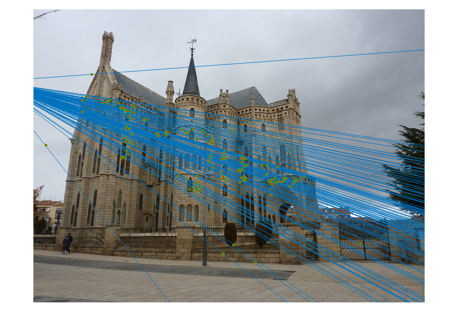
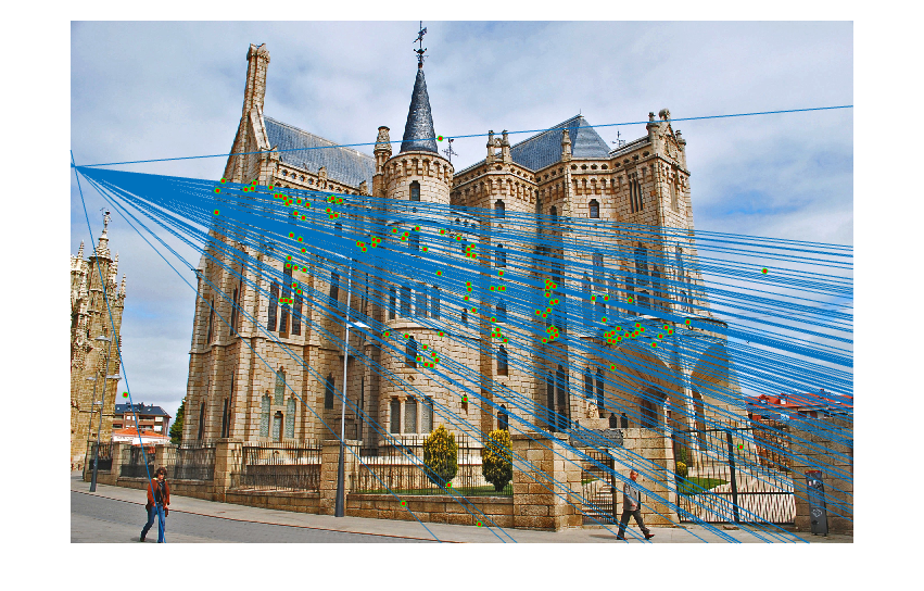
The first part of the code normalizes the points by subtracting the mean and dividing by the standard deviation to prevent issues with poor numerical conditioning when computing the fundamental matrix. The A matrix is then created to represent the system of equations AF = 0. This matrix is used to solve for F using SVD. To enforce the singularity constraint, the last singular value of the F matrix is zeroed. Finally, the F matrix is transformed back to its original units using the inverse of the transform applied to the input points. Running this algorithm on the same image pair as the previous section yields the following epipolar lines and fundamental matrix:
 |
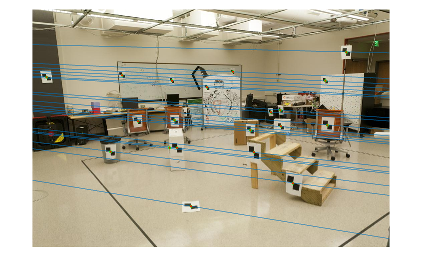 |
F_matrix =

    0.0000   -0.0000    0.0007
   -0.0000    0.0000   -0.0054
    0.0000    0.0074   -0.1716
As shown in the images above, the epipolar lines corresponding to the fundamental matrix intersect with each matched point in the two images.
Part III
For the final part of this project, the same fundamental matrix estimation code is used along with RANSAC to determine which keypoint matches are valid inliers on three pairs of images (Mount Rushmore, Notre Dame, and Episcopal Gaudi). This code was implemented in the ransac_fundamental_matrix() Matlab function, shown below:
N = 100000;
delta = 0.01;
s = 8;

% RANSAC loop
num_inliers = -1;
for i = 1:N
    % Randomly sample s points
    inds = randsample(size(matches_a,1),s);

    % Find F matrix using these points
    F = estimate_fundamental_matrix(matches_a(inds,:), matches_b(inds,:));

	% Compute distance between each point and model x^TFx'=0 for perfect
    dists = sum(([matches_a, ones(size(matches_a,1), 1)] * F) .* [matches_b, ones(size(matches_b,1), 1)], 2);

    % Find inliers - if greater than num_inliers, update best F and inliers
    inliers = abs(dists) <= delta;
    if sum(inliers) > num_inliers
        num_inliers = sum(inliers);
        inliers_a = matches_a(inliers,:);
        inliers_b = matches_b(inliers,:);
        Best_Fmatrix = estimate_fundamental_matrix(inliers_a, inliers_b);
    end
end
The RANSAC code begins by defining several parameters. The "N" parameter determines the number of iterations of RANSAC that will be run. Generally, the larger this number, the better the fundamental matrix estimation will be. With 100,000 iterations, the program terminates in a few seconds and typically produces good estimates of the fundamental matrix. The second parameter is delta, which is the maximum error for a point to be considered an inlier. Smaller values of delta will be more selective and will produce fewer but better point correspondences. Through some testing, the value of 0.01 was found to effectively eliminate most outliers. The final parameter, s, is the number of points to sample. This value was set to 8 because this is the minimum number of points needed to calculate the fundamental matrix estimation.
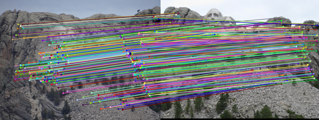
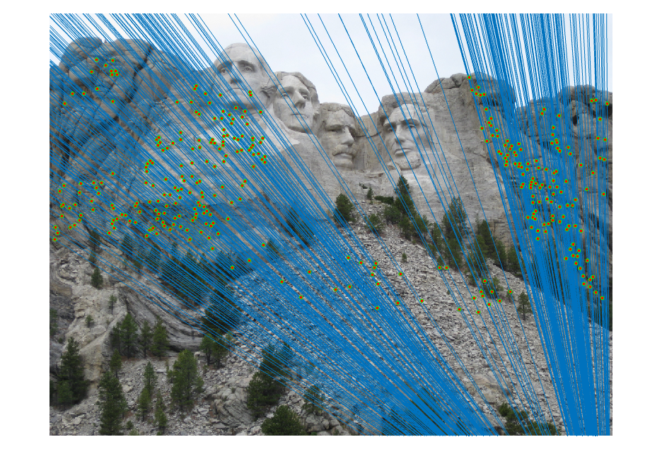
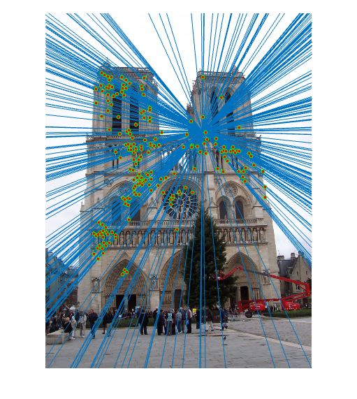
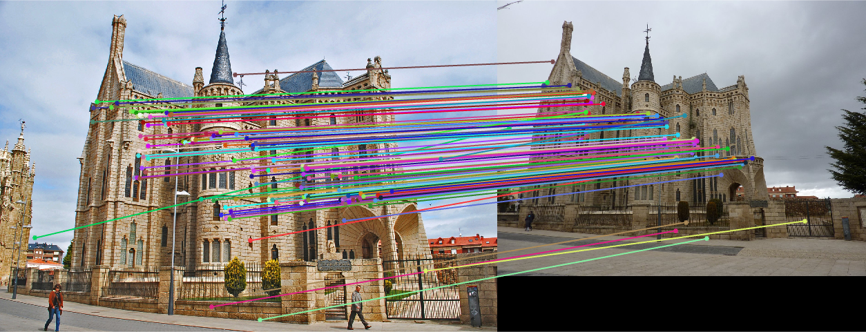
The next part of the code runs each iteration of the RANSAC loop. In each iteration, 8 points are sampled at random and these points are used to estimate the fundamental matrix. Using this fundamental matrix, the distance between each point correspondence and F is computed, where distance is defined as the value of xTFx', which will be zero if the points are a perfect correspondence. The number of inliers with respect to this distance are then determined, and if the number of inliers is the new maximum, these inliers are recorded. In this case, the fundamental matrix is re-estimated using all of the inlier points to produce a more accurate estimate. Shown below are the results of running this algorithm on each of the three image sets, including the inlier point correspondences and the epipolar lines:
 |
|
 |
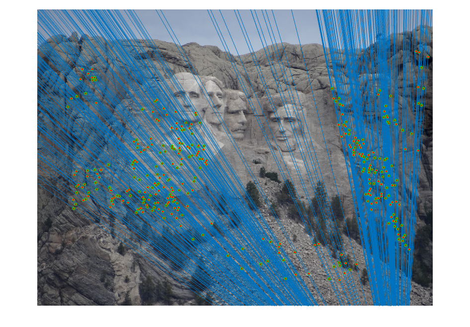 |
| Mount Rushmore inliers and epipolar lines | |
 |
|
 |
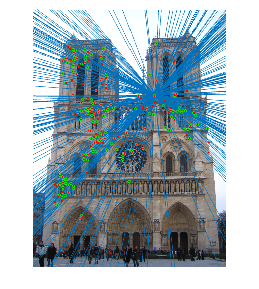 |
| Notre Dame inliers and epipolar lines | |
 |
|
 |
 |
| Episcopal Gaudi inliers and epipolar lines | |
For the first two image sets, the algorithm is able to find a large number of inlier correspondences, nearly all of which are correct matches. The performance on the Episcopal Gaudi pair is not as strong as the other two; there are not as many point correspondences found, and several of these are incorrect. However, most of the matches are still correct.