Project 3 / Camera Calibration and Fundamental Matrix Estimation with RANSAC
For information regarding the specifics of calculations and specifications please see the assignment details here
Basic Steps
- Camera Projection Matrix
- Fundamental Matrix Estimation
- Fundamental Matrix with RANSAC
- Normalization add-on to Fundamental Matrix (Extra Credit)
Camera Projection Matrix
In order to approximate the projection matrix we needed a list of 2D and 3D points and their correspondences. Luckily we were given these points by the problem spec. Once we had these points we can simply set up a system of linear equations and solve for the missing terms that are the elements of the projection matrix. In order to do this we set up the following formula and solved for M (which is a reshaped version of the projection matrix).
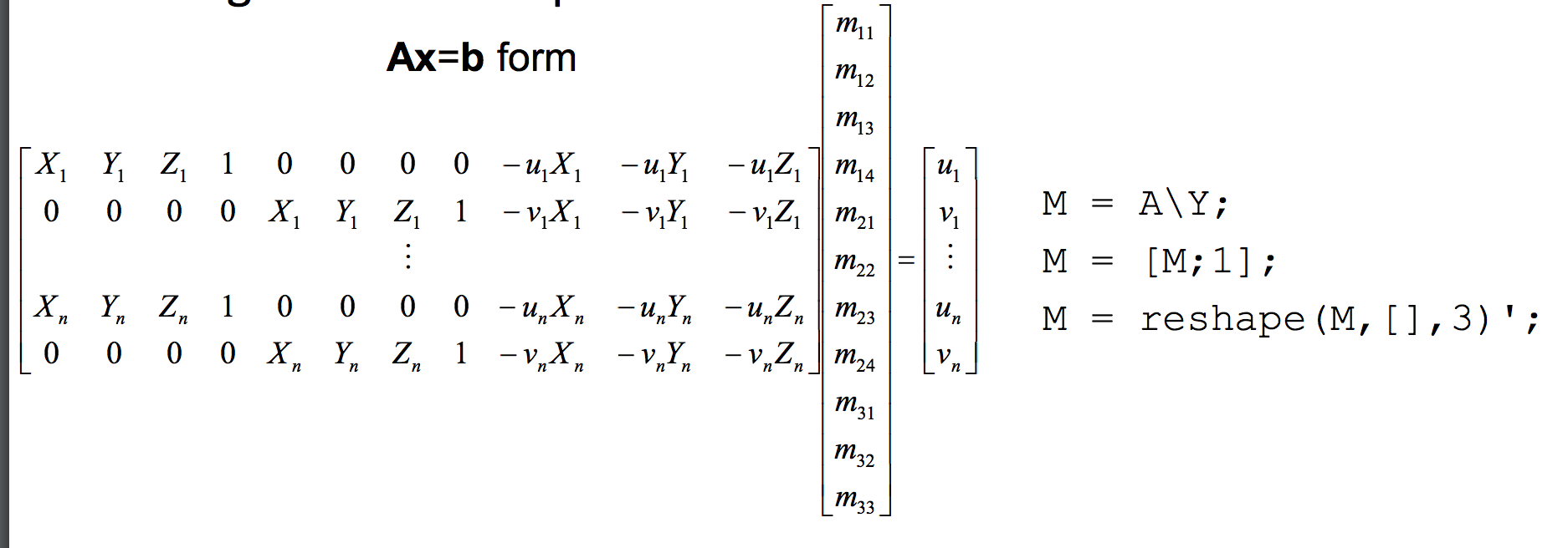
(image taken from slide 37 in slide-deck at http://www.cc.gatech.edu/~hays/compvision/lectures/13.pdf)
From this we were able to compute the camera center by using the formula we derived in class that
Fundamental Matrix Estimation
In order to approximate the fundamental matrix we needed 2 lists of 2D points in different images (believed to have correspondence) and then we could perform a regression to solve for
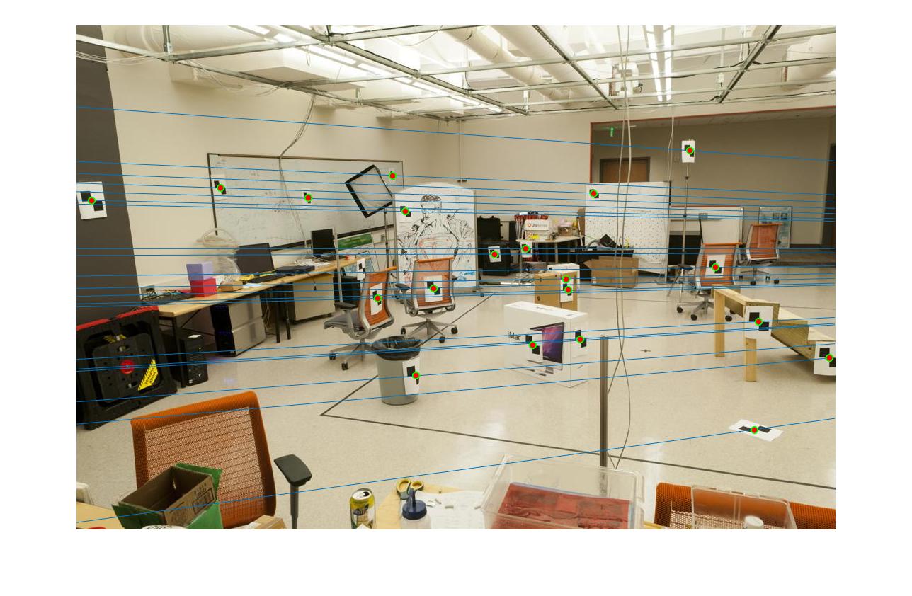
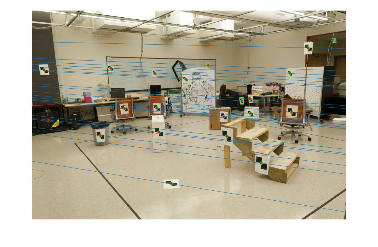
similar to the process we used in part 1. However the fundamental matrix is rank 2, so as an additional step we perform SVD and remove the smallest eigenvalue (set it to zero). Once we had our estimated fundamental matrix we could measure our correctness by looking at the epipolar lines between the images. Note that all interest points should have lines going directly through them in a perfect world.
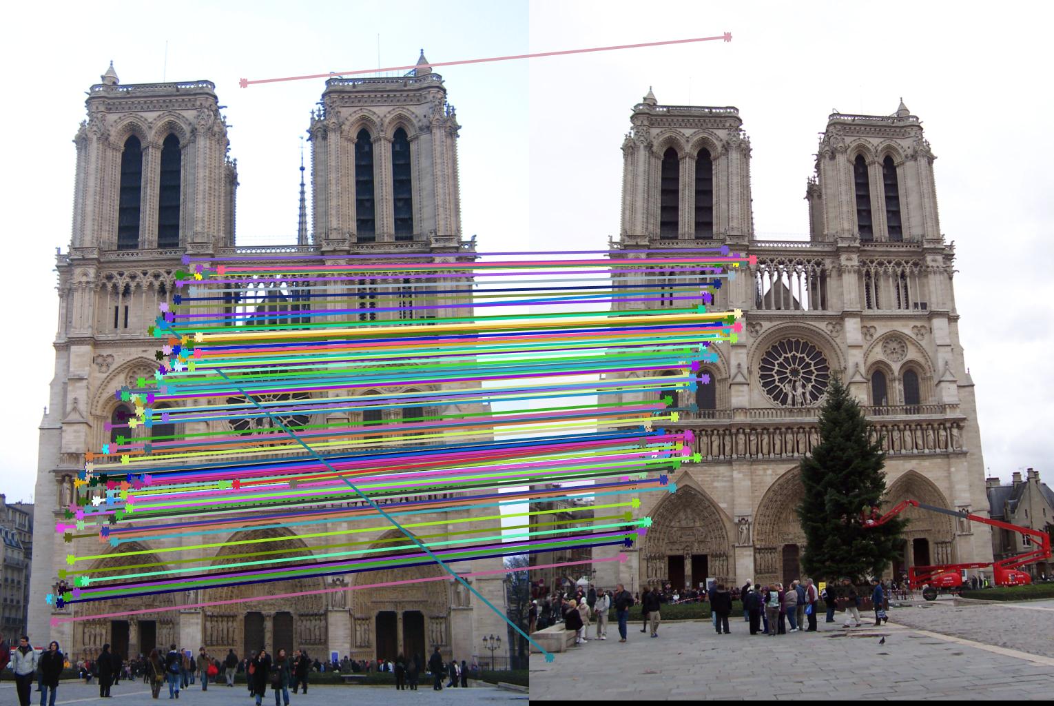
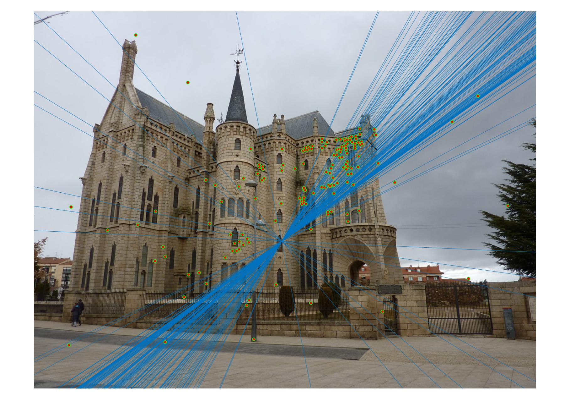
Fundamental Matrix with RANSAC
While this correspondence looked perfect in part 2 this was because all of our interest points were already correctly matched. In reality we have many false points and would like to still be able to estimate the fundamental matrix. In order to do this we used the RANSAC algorithm which is a fancy way of saying we:
- estimated the fundamental matrix based on a small number of interest points
- measured how many other interest points agreed with this model
- repeat (1000s of times) only keeping the best result (has the most points that agree with it)
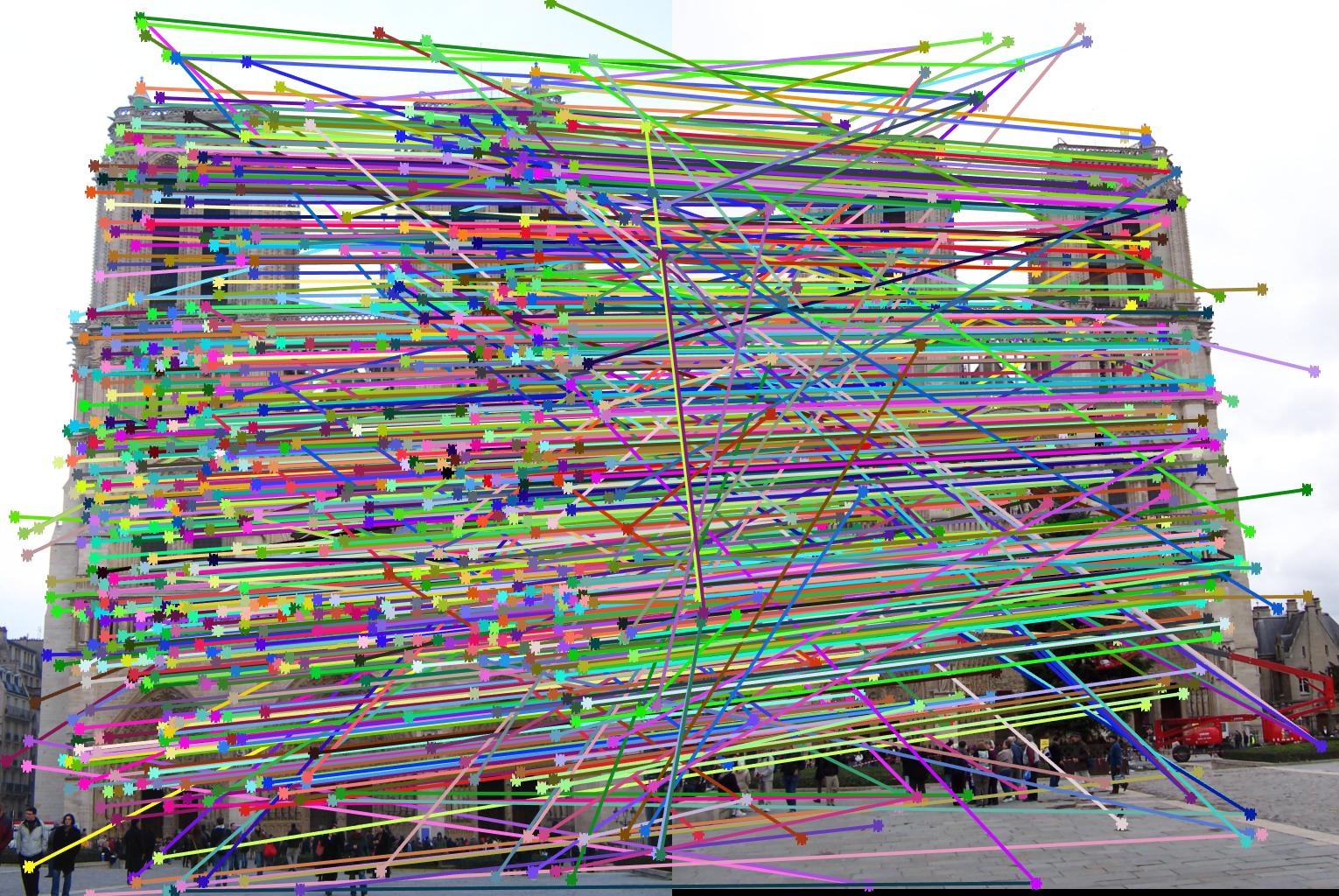
This allowed us to eliminate more spurious interest points creating more meaningful matchings between interest points as seen below.
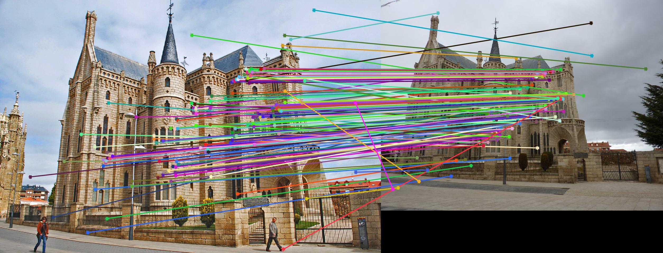
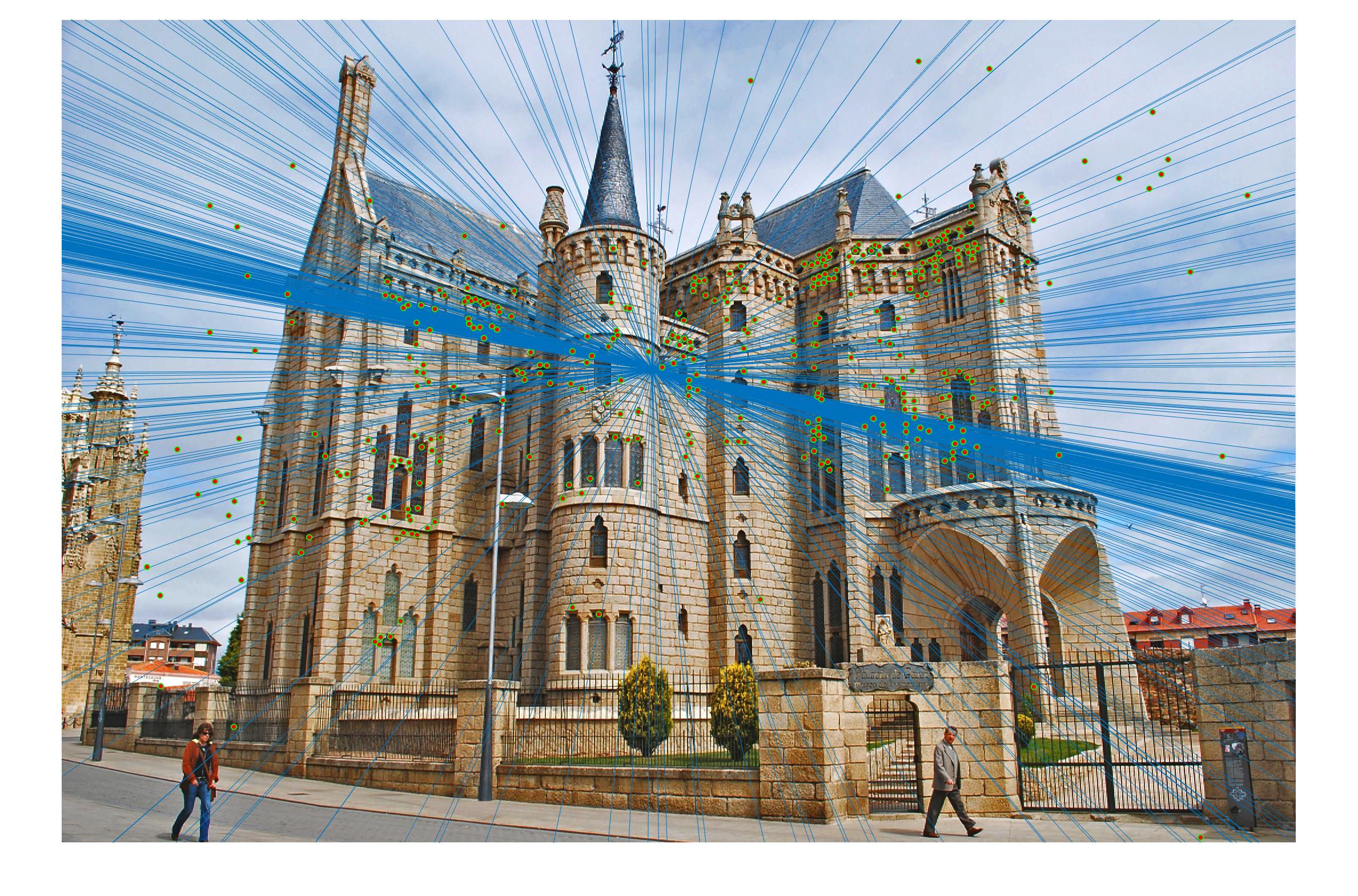
Normalization add-on to Fundamental Matrix (Extra Credit)
We can further increase the accuracy of the estimation of the fundamental matrix by normalizing the coordinates before solving for the fundamental matrix. To do this we:
- found the maximum absolute value and divide all elements by that value. (This makes the regression less influenced by large values).
- perform the regression as before (part 2)
- transform the matrix back to the correct scale.
For more information on how this was done please look in the estimate_fundamental_matrix.m file or in the design doc listed at the top.
Normalization allowed us to eliminate more spurious interest points creating more meaningful matchings between interest points as seen below.
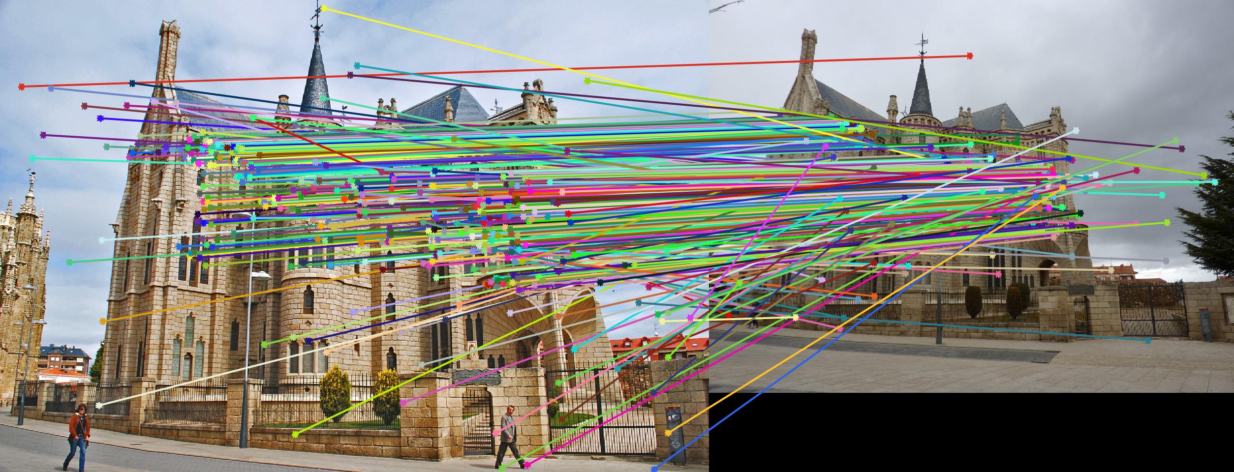
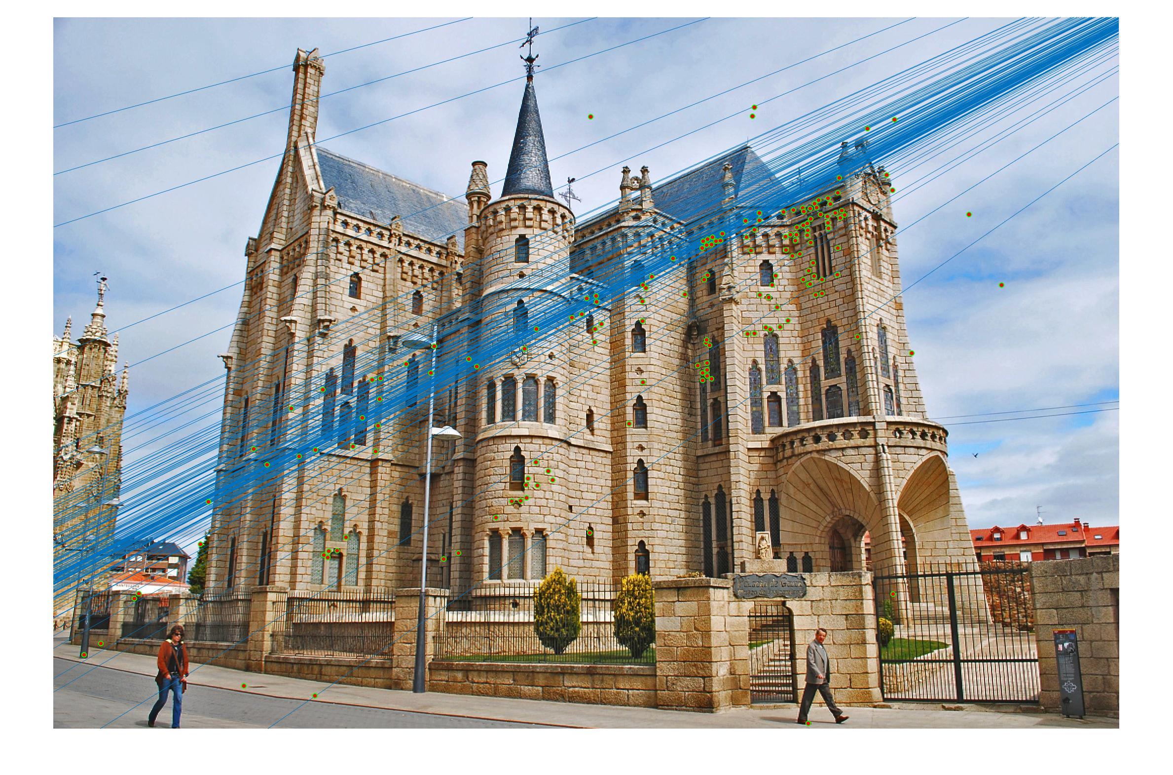
It is also easier to see the correctness that we gain by looking at the epipolar lines.
Epipolar lines visualization before and after normalization
| Before |
|
| After |
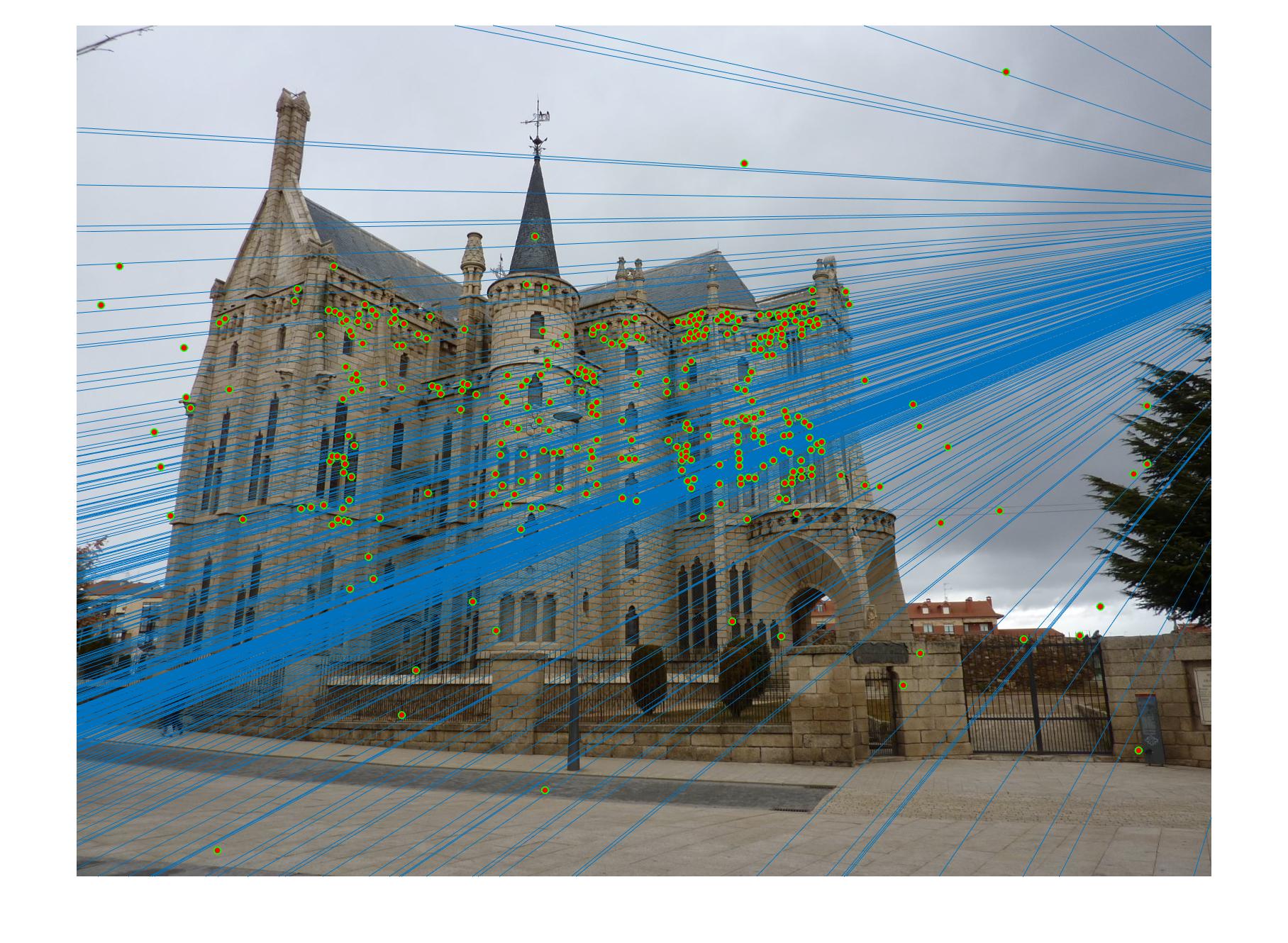
|