Project 3: Camera Calibration and Fundamental Matrix Estimation with RANSAC
The goal of this project was to estimate the camera projection matrix and fundamental matrix between a pair of images.
Part I: Camera Projection Matrix
The projection matrix M transforms 3D world coordinates to 2D image coordinates. This was done by constructing a system of homogeneous linear equations from each pair of corresponding 2D <ui, vi> and 3D <Xi, Yi, Zi> coordinates:
| X1 | Y1 | Z1 | 1 | 0 | 0 | 0 | 0 | -u1X1 | -u1Y1 | -u1Z1 | -u1 |
| 0 | 0 | 0 | 0 | X1 | Y1 | Z1 | 1 | -v1X1 | -v1Y1 | -v1Z1 | -v1 |
| ... | |||||||||||
| Xn | Yn | Zn | 1 | 0 | 0 | 0 | 0 | -unXn | -unYn | -unZn | -un |
| 0 | 0 | 0 | 0 | Xn | Yn | Zn | 1 | -vnXn | -vnYn | -vnZn | -vn |
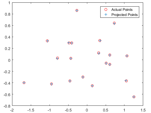
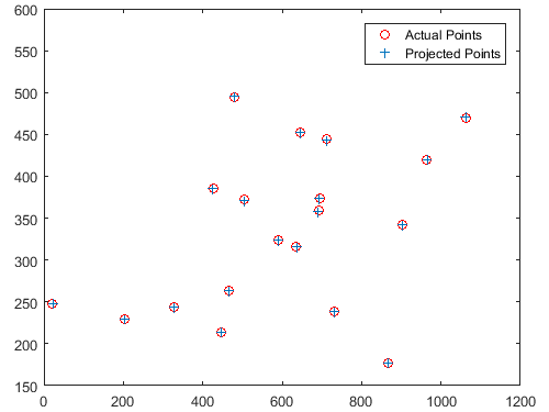
Total residual of the estimated projection matrix = 0.0445
This system of homogeneous linear equations was then solved using linear least squares. In MATLAB, the singular value decomposition was performed on the constructed matrix. The final estimated projection matrix M is the last column in the resulting V matrix, reshaped into a 3x4 matrix. From the given normalized point data, this computes to:
| 0.4583 | -0.2947 | -0.0140 | 0.0040 |
| -0.0509 | -0.0546 | -0.5411 | -0.0524 |
| 0.1090 | 0.1783 | -0.0443 | 0.5968 |
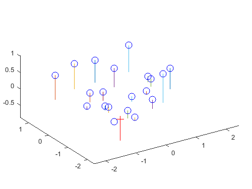
The red cross represents the camera center. The blue circles represent the given interest points.
Next, the camera center was computed from the estimated projection matrix. This is done with a few simple matrix operations:
C = -Q-1m4
where Q is the 3x3 submatrix M1-3,1-3, and m4 is the column vector M1-3,4. From the given normalized point data, the camera center C is estimated to be at <-1.5127, -2.3517, 0.2826>.
With the more difficult, non-normalized point data, the estimated projection matrix was:
| 0.0069 | -0.0040 | -0.0013 | -0.8267 |
| 0.0015 | 0.0010 | -0.0073 | -0.5625 |
| 0.0000 | 0.0000 | -0.0000 | -0.0034 |
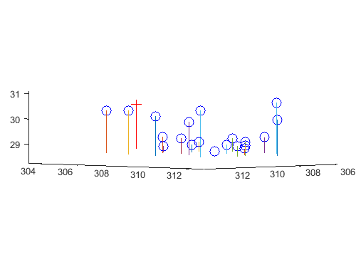
Total residual = 15.5450. Camera center = <303.1000, 307.1843, 30.4217>.
Part II: Fundamental Matrix Estimation
The fundamental matrix F is used to estimate the mapping of points in one image to lines in another image. This was accomplished with the eight-point algorithm in a very similar manner as explained in Part I, where a system of homogeneous linear equations was constructed from corresponding 2D coordinates in each image <ui, vi> and <ui', vi'>:
| u1u1' | u1v1' | u1 | v1u1' | v1v1' | v1 | u1' | v1' | 1 |
| ... | ||||||||
| unun' | unvn' | un | vnun' | vnvn' | vn | un' | vn' | 1 |
Again, this was solved by performing the singular value decomposition on the constructed matrix. The last column of the resulting V matrix was then reshaped into a 3x3 matrix and transposed to form the fundamental matrix F. Finally, the rank 2 constraint was enforced to make the epipolar lines coincident. Another singular value decomposition was performed on F, and S3,3 was set to 0 before finalizing F:
F = U * S * VT
As a result, the fundamental matrix for the sample image pair was estimated to be:
| -0.0000 | 0.0000 | -0.0019 |
| 0.0000 | 0.0000 | 0.0172 |
| -0.0009 | -0.0264 | 0.9995 |

Fundamental matrix with added noise:
| -0.0000 | 0.0000 | -0.0005 |
| 0.0000 | 0.0000 | 0.0060 |
| -0.0013 | -0.0133 | 0.9999 |
These results were improved, however, by centering and normalizing the point data before using the eight-point algorithm to compute the fundamental matrix F. For each image, transformation matrices Ta and Tb were constructed to scale the point data by s such that the mean distance from each point to the origin is √2 and center the point data on its centroid cu,v:
| s | 0 | -scu |
| 0 | s | -scv |
| 0 | 0 | 1 |
Finally, the fundamental matrix was transformed back to its original units:
Forig = TbT * Fnorm * Ta
Normalized fundamental matrix:
| -0.0000 | 0.0000 | -0.0002 |
| 0.0000 | -0.0000 | 0.0013 |
| -0.0000 | -0.0018 | 0.0411 |

Normalized fundamental matrix with added noise:
| -0.0000 | 0.0000 | -0.0001 |
| 0.0000 | 0.0000 | 0.0012 |
| -0.0000 | -0.0018 | 0.0676 |

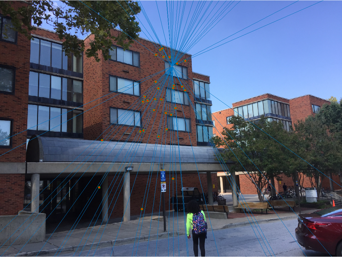
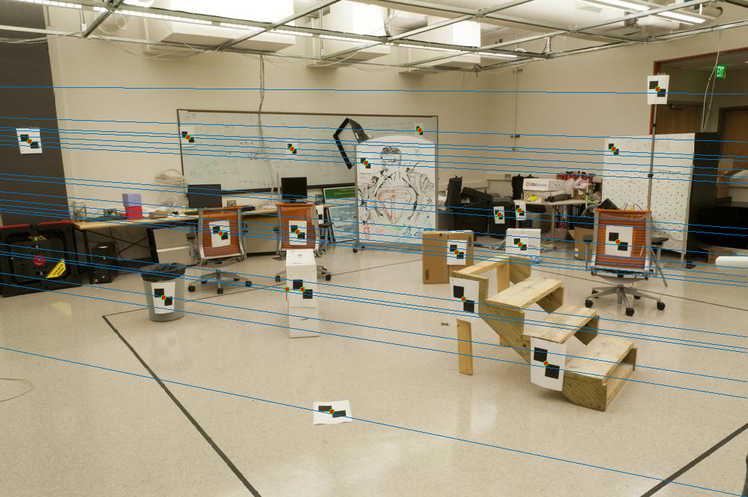
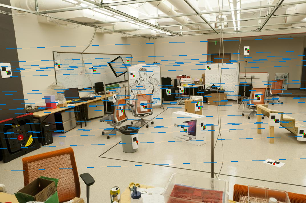
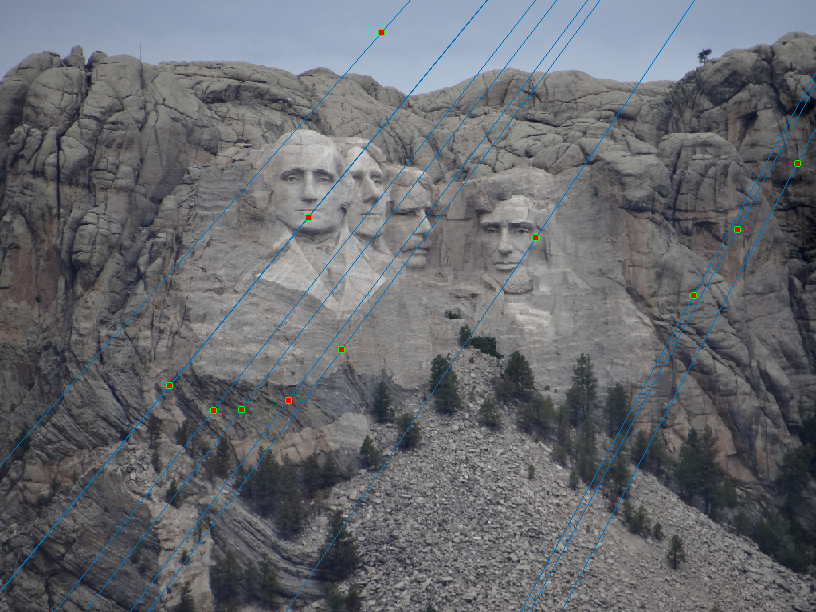
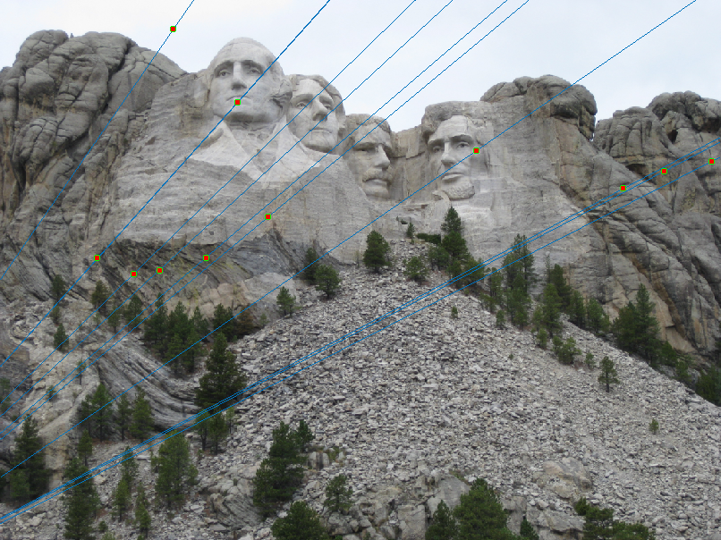
Part III: Fundamental Matrix with RANSAC
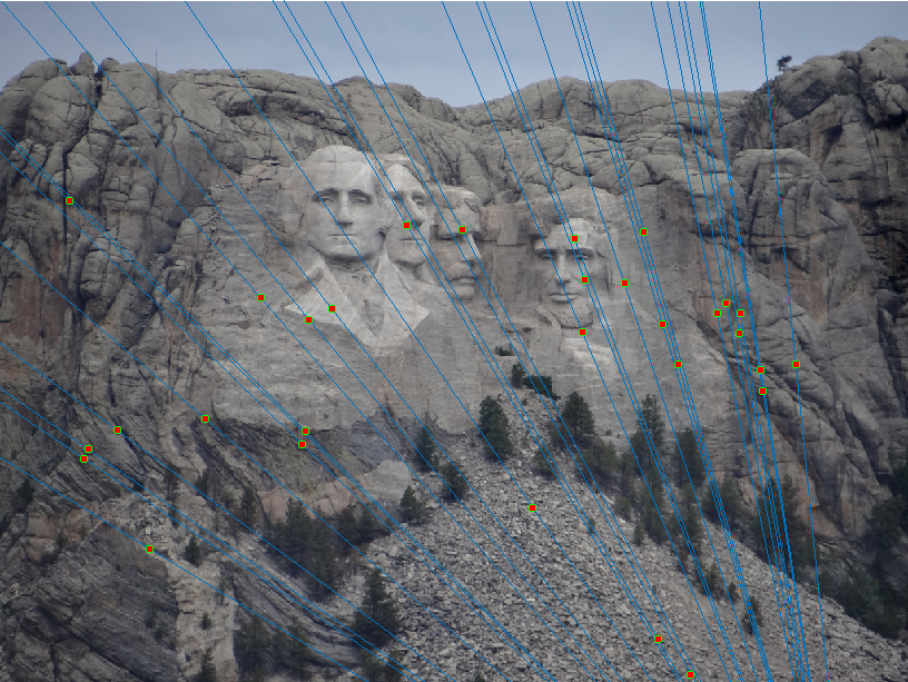
In Part II, perfect point correspondences were already given to estimate the fundamental matrix. The goal for this part is to estimate the fundamental matrix F on any pair of images with RANSAC, where we do not already have perfect point correspondences. We begin with a list of potentially spurious point correspondences from VLFeat's SIFT feature detector. For an arbitrary number of loops (3000 in this case, but more is generally better at the cost of compute time), a random sample of 8 point correspondences are taken and used to estimate the fundamental matrix using the method described in Part II. In each iteration, inliers were determined based on a distance metric:
distance = <ui', vi', 1> * F * <ui, vi, 1>T
A distance threshold ε = 0.0001 was then tested against the rest of the potential point correspondences and used to include only inliers with distance less than ε. A range of values were tested for ε. However, it was found that higher values led to significantly more inliers, but many of those inliers were incorrect. On the other hand, lower values led to fewer inliers, but they seemed to be more correct. ε = 0.0001 was chosen because it consistently gave a reasonable number (a few dozen) of inliers across most test cases. Finally, the confidence for each iteration of RANSAC was rated by the percentage of inliers found in the point correspondences. After 3000 iterations, the iteration with the most confident results were returned, and the best fundamental matrix was recalculated based only on the most confident inliers.
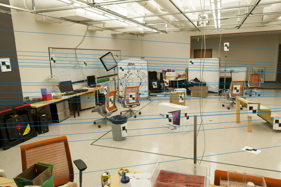
Results without Normalization
Mount Rushmore
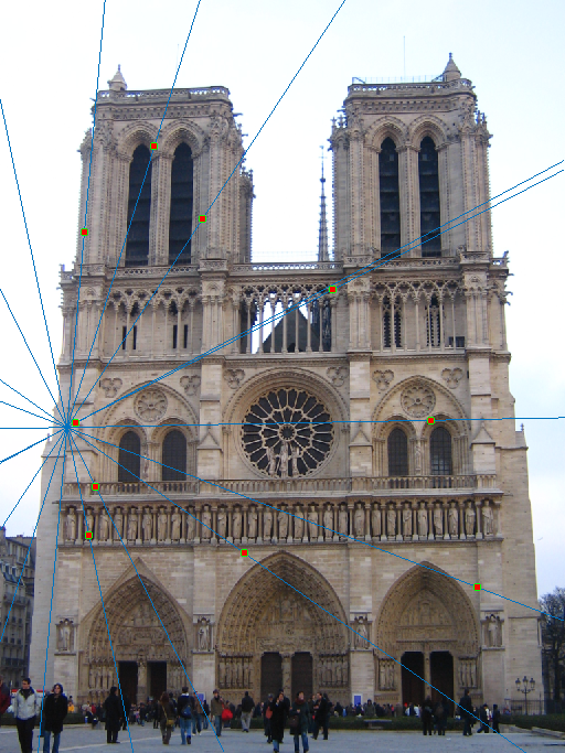
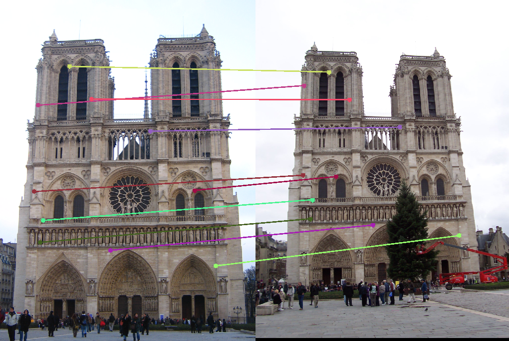
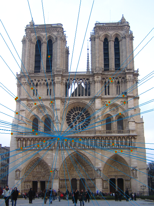
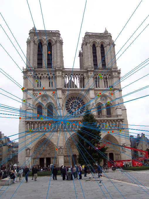
Notre Dame
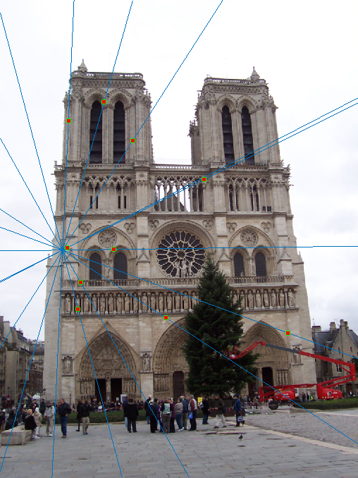
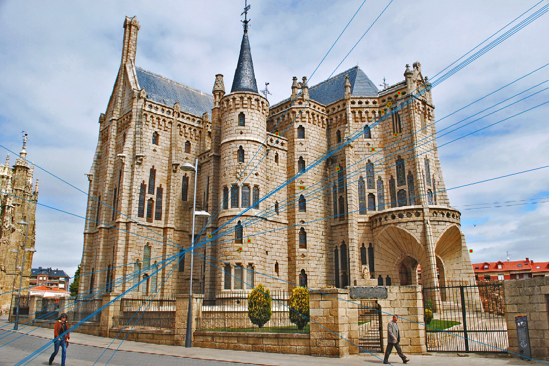
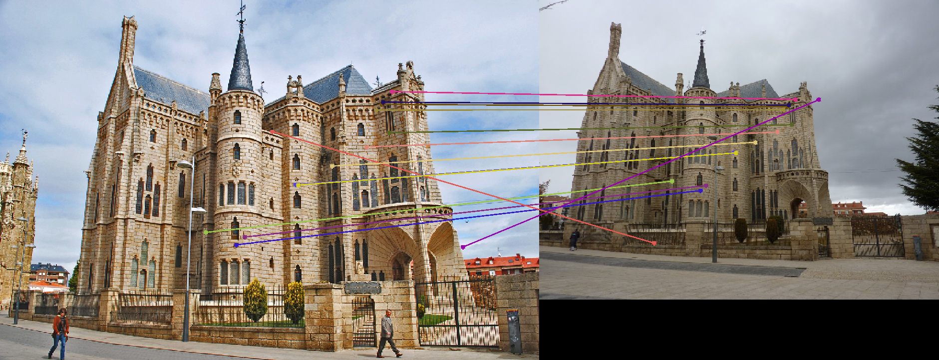
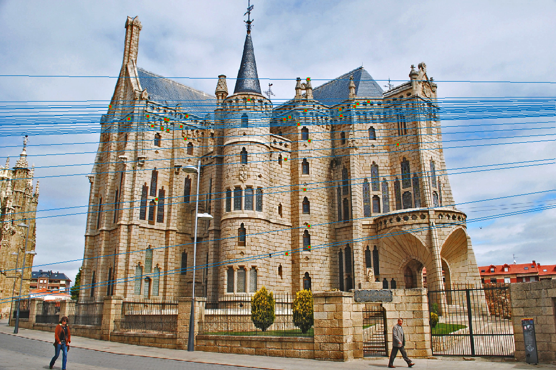
Episcopal Gaudi
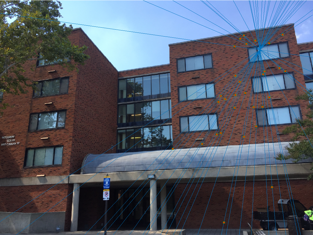
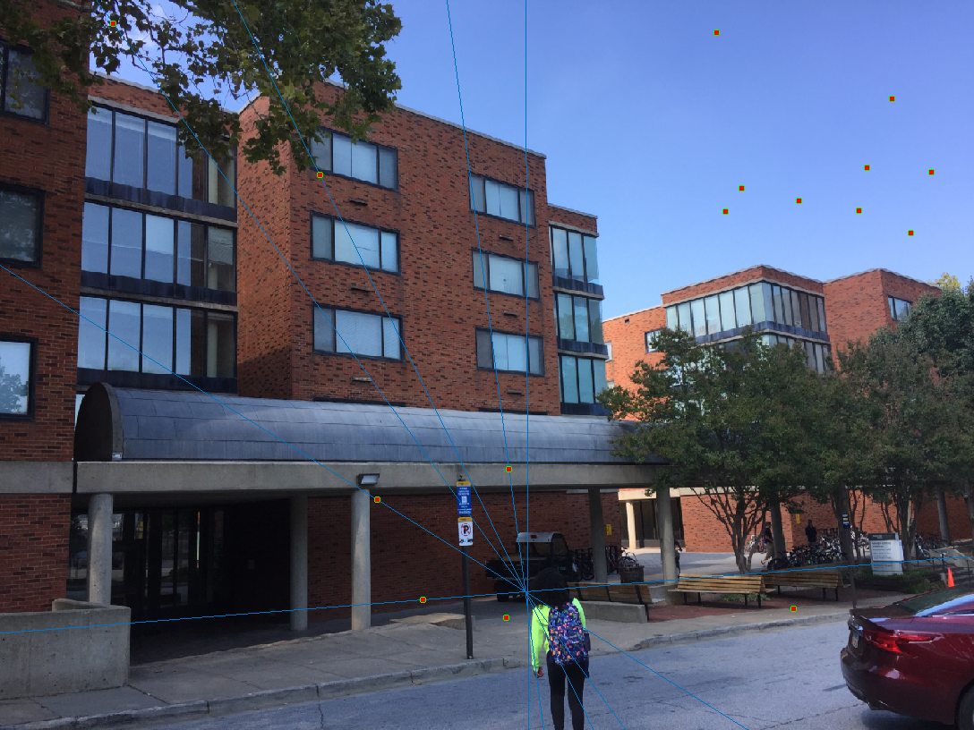
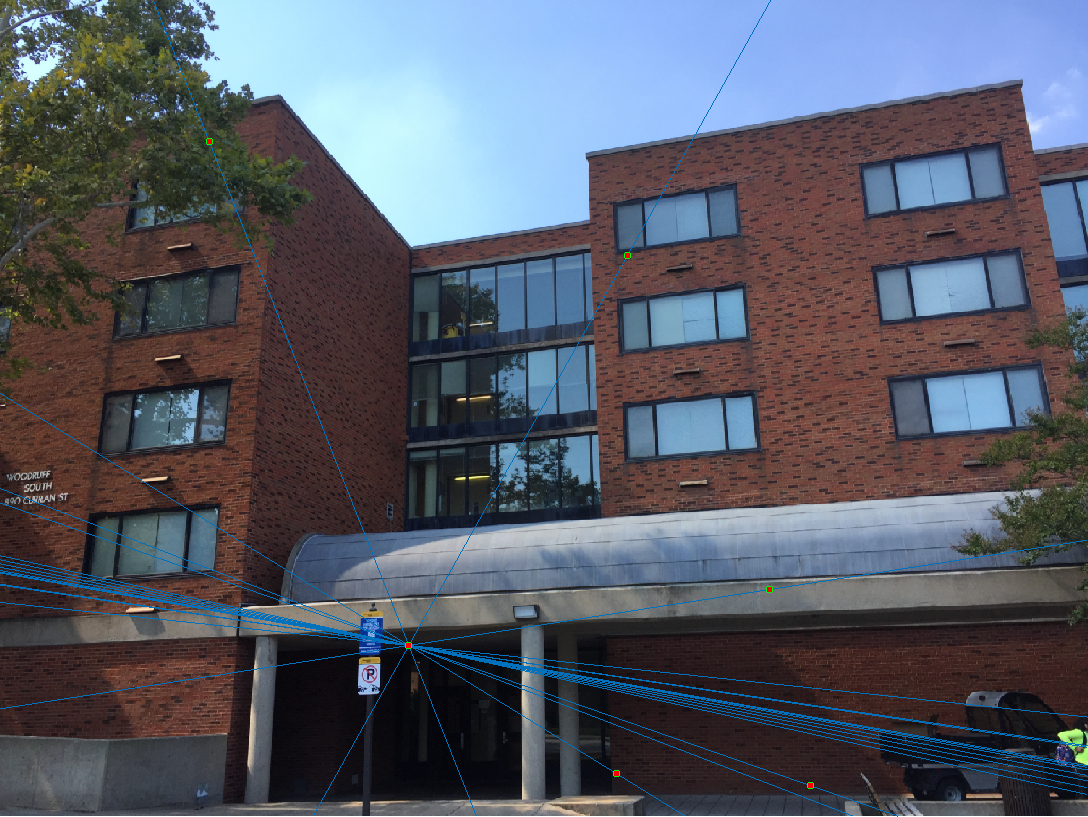
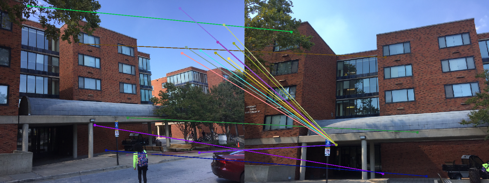
Woodruff
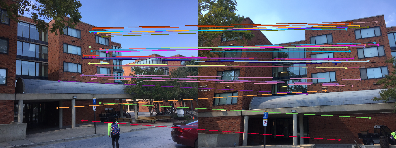
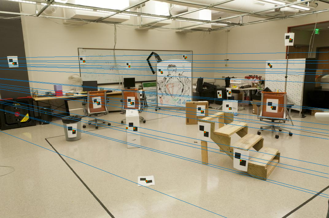
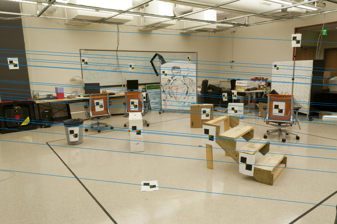
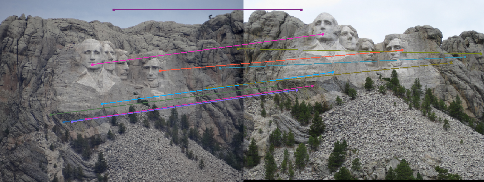
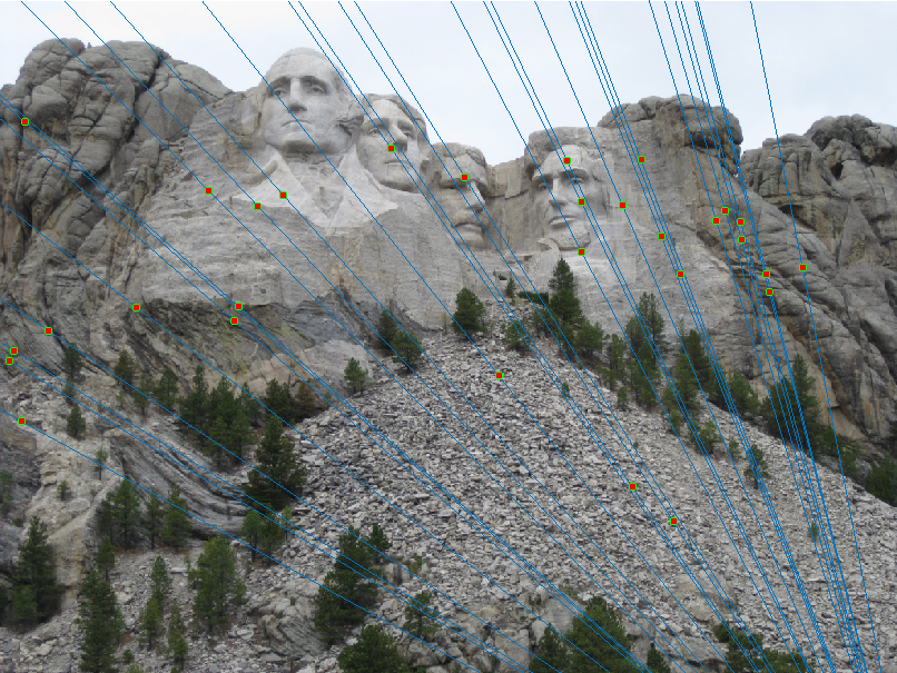
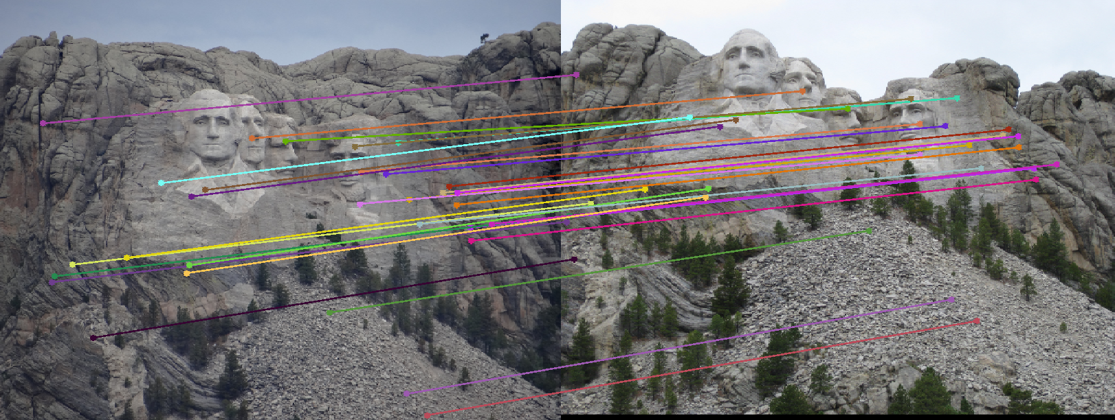
Results with Normalization
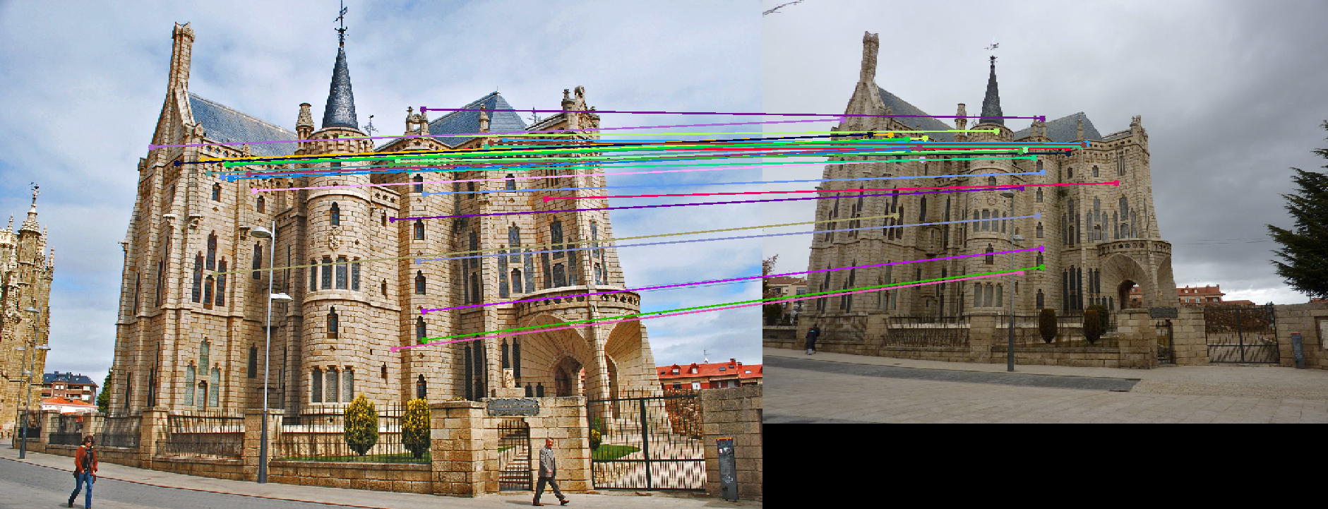
(Note: For clarity, only 30 randomly selected point correspondences are displayed in the results below.)
Mount Rushmore
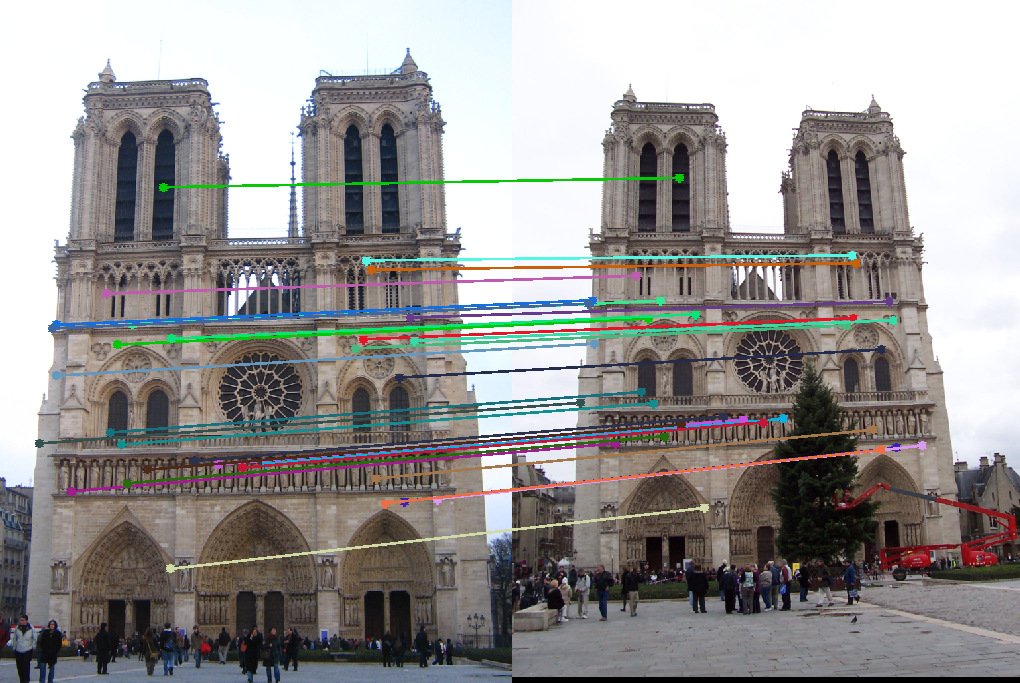
Notre Dame
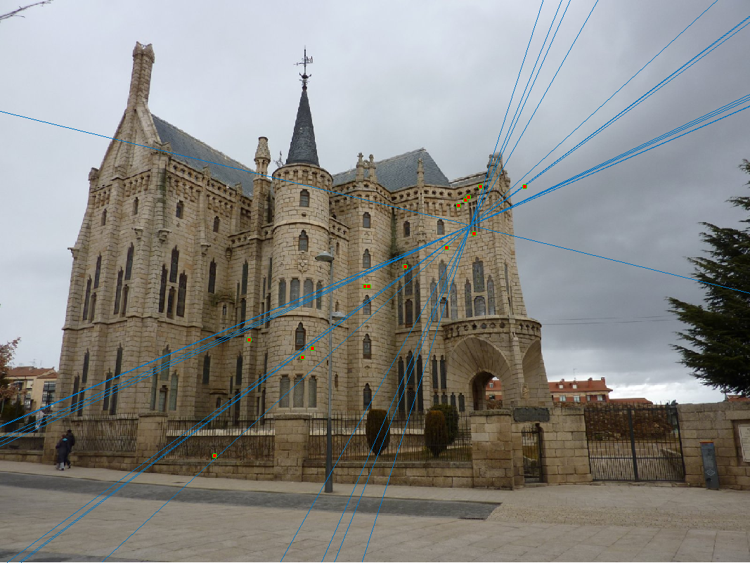
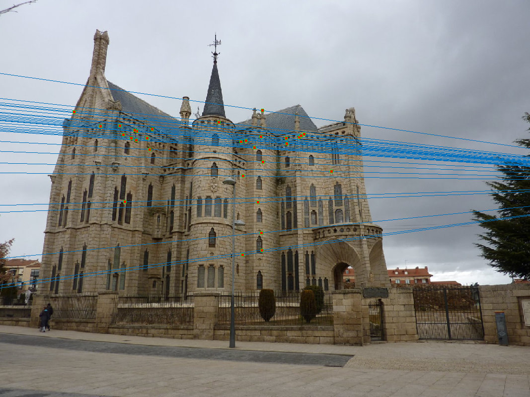
Episcopal Gaudi
Woodruff