Jingdao Chen

Project 3 / Camera Calibration and Fundamental Matrix Estimation with RANSAC

Camera Projection Matrix

To find the camera projection matrix M, a series of linear equations is set up as shown below using the corresponding 2D and 3D points. Since the matrix is only defined up to a scale, the last element is fixed at one and the remaining elements are solved using least-squares.

%code for M matrix

%                                                     [M11       [ u1
%                                                      M12         v1
%                                                      M13         .
%                                                      M14         .
%[ X1 Y1 Z1 1 0  0  0  0 -u1*X1 -u1*Y1 -u1*Z1          M21         .
%  0  0  0  0 X1 Y1 Z1 1 -v1*Z1 -v1*Y1 -v1*Z1          M22         .
%  .  .  .  . .  .  .  .    .     .      .          *  M23   =     .
%  Xn Yn Zn 1 0  0  0  0 -un*Xn -un*Yn -un*Zn          M24         .
%  0  0  0  0 Xn Yn Zn 1 -vn*Zn -vn*Yn -vn*Zn ]        M31         .
%                                                      M32         un
%                                                      M33         vn ]

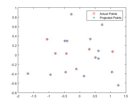
The results for calculation of projection matrix are shown below:

%result for M matrix

The projection matrix is:
    0.7679   -0.4938   -0.0234    0.0067
   -0.0852   -0.0915   -0.9065   -0.0878
    0.1827    0.2988   -0.0742    1.0000


The total residual is: <0.0445>

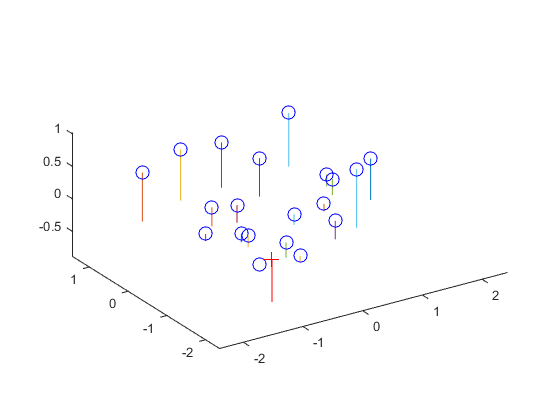
Furthermore, the camera center can be extracted from the M matrix using the formula: C = - Q^-1 m₄. The results are shown below:

%result for camera center

The estimated location of camera is: <-1.5126, -2.3517, 0.2827>

Fundamental Matrix Estimation

The fundamental matrix, F is used to relate point pairs across two images. A series of 8 or more linear equations is set up and Singular Value Decomposition (SVD) is used to find the vector corresponding to the smallest singular value. To reduce the rank of F, the smallest singular value is set to zero and a new estimate of F is generated using multiplication of the SVD matrices.

%result for fundamental matrix

F_matrix =

   -0.0000    0.0000   -0.0019
    0.0000    0.0000    0.0172
   -0.0009   -0.0264    0.9995

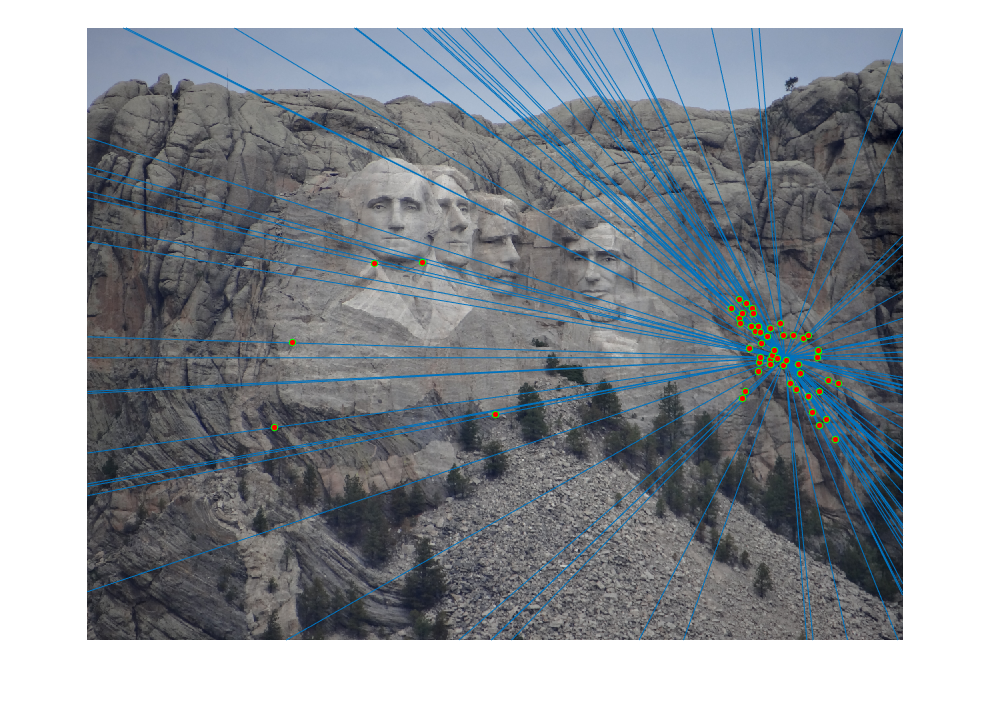
The epipolar lines resulting from the estimated fundamental matrix can be visualized as follows:

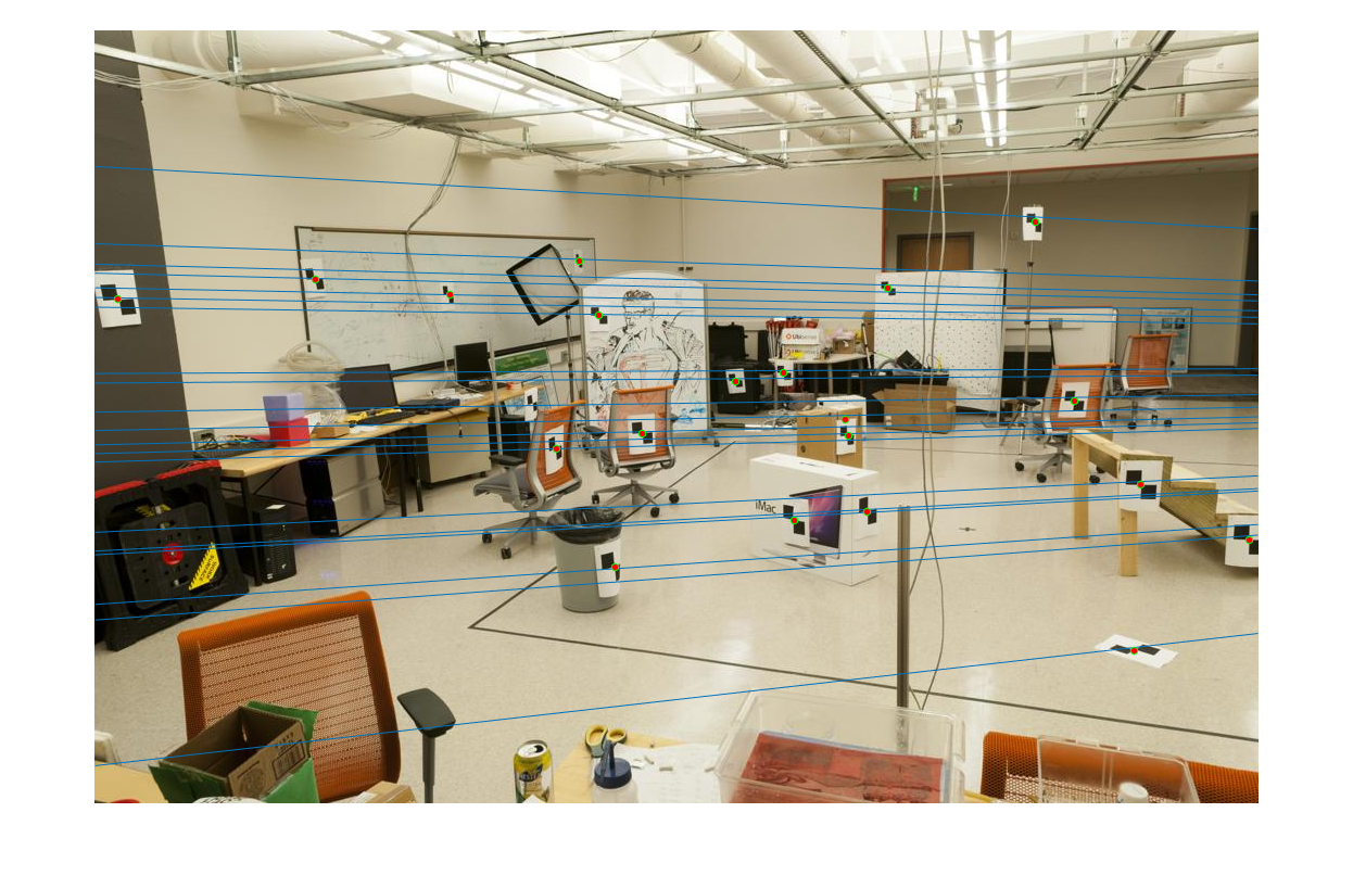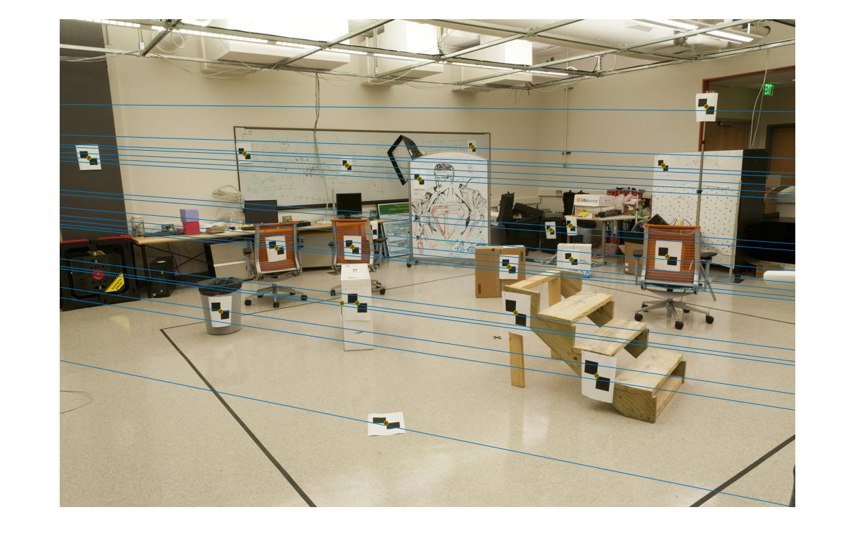Fundamental Matrix with RANSAC

The RANSAC algorithm is used to improve the estimation of fundamental matrix given potentially incorrect point correspondences. The RANSAC algorithm is implemented as shown below with the number of iterations set to 1000 and the error threshold set to 0.001.

%RANSAC algorithm

for iter=1:numIter
    id = randi(N,8,1);
    pointsA = matches_a(id,:);
    pointsB = matches_b(id,:);
    F = estimate_fundamental_matrix(pointsA, pointsB);
    score = sum(homogenousB*F.*homogenousA,2);
    numInliers = nnz(abs(score) maxInliers)
        Best_Fmatrix = F;
    end
end

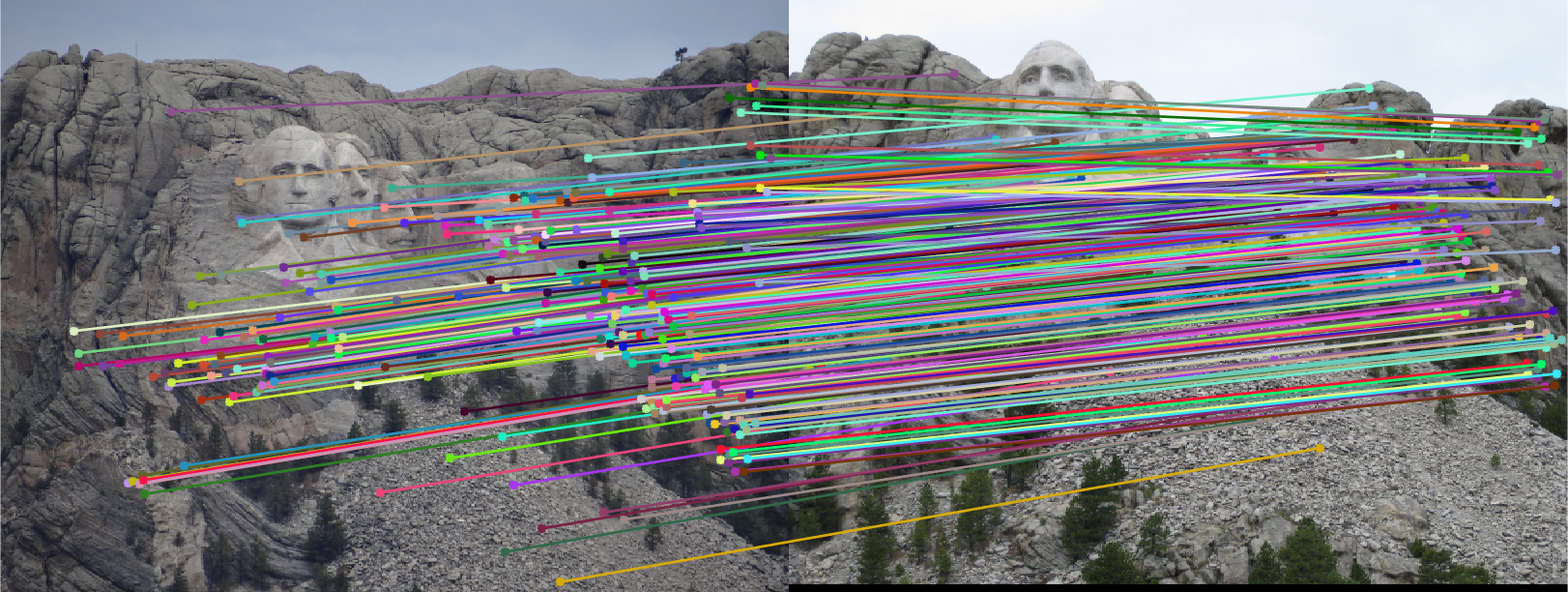
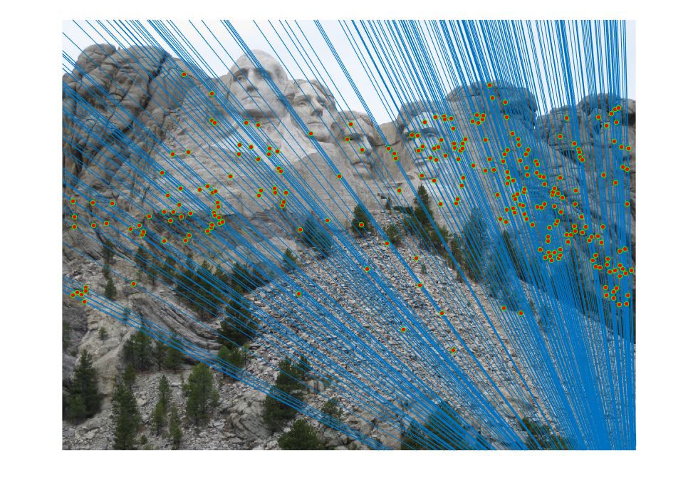
The initial matches, corrected matches, and epipolar lines plot are shown below:

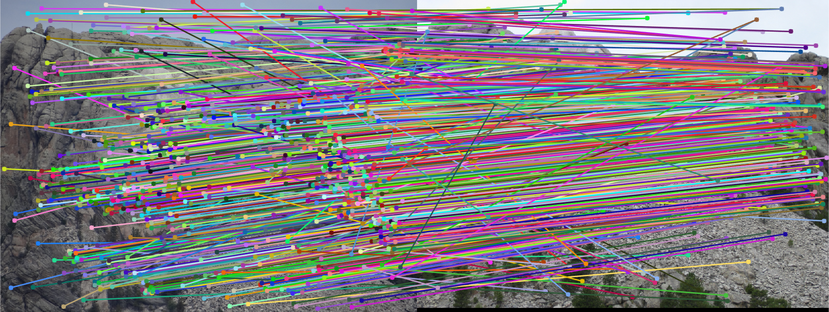
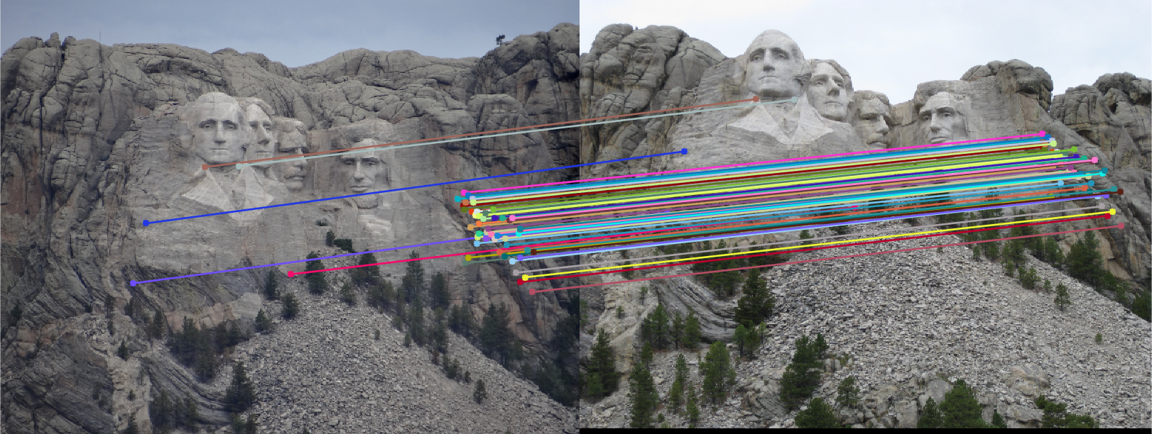
Extra Credit

The overcome the problem of having an ill-constrained matrix when estimating F, the image coordinates are first normalized according to the following scheme:

%normalization

function [Ta,Tb,newA,newB] = normalizePoints(pointsA,pointsB)
    cu = mean(pointsA(:,1));
    cv = mean(pointsA(:,2));
    s = 1 / std([pointsA(:,1)-cu;pointsA(:,2)-cv]);
    Ta = [s 0 0 ;0 s 0;0 0 1] * [1 0 -cu;0 1 -cv;0 0 1];
    newA = [(pointsA(:,1)-cu)*s,(pointsA(:,2)-cv)*s];
    cu = mean(pointsB(:,1));
    cv = mean(pointsB(:,2));
    s = 1 / std([pointsB(:,1)-cu;pointsB(:,2)-cv]);
    Tb = [s 0 0 ;0 s 0;0 0 1] * [1 0 -cu;0 1 -cv;0 0 1];
    newB = [(pointsB(:,1)-cu)*s,(pointsB(:,2)-cv)*s];
end

[Ta,Tb,pointsA,pointsB] = normalizePoints(pointsA,pointsB);
F = estimate_fundamental_matrix(pointsA, pointsB);
F = Tb' * F * Ta;

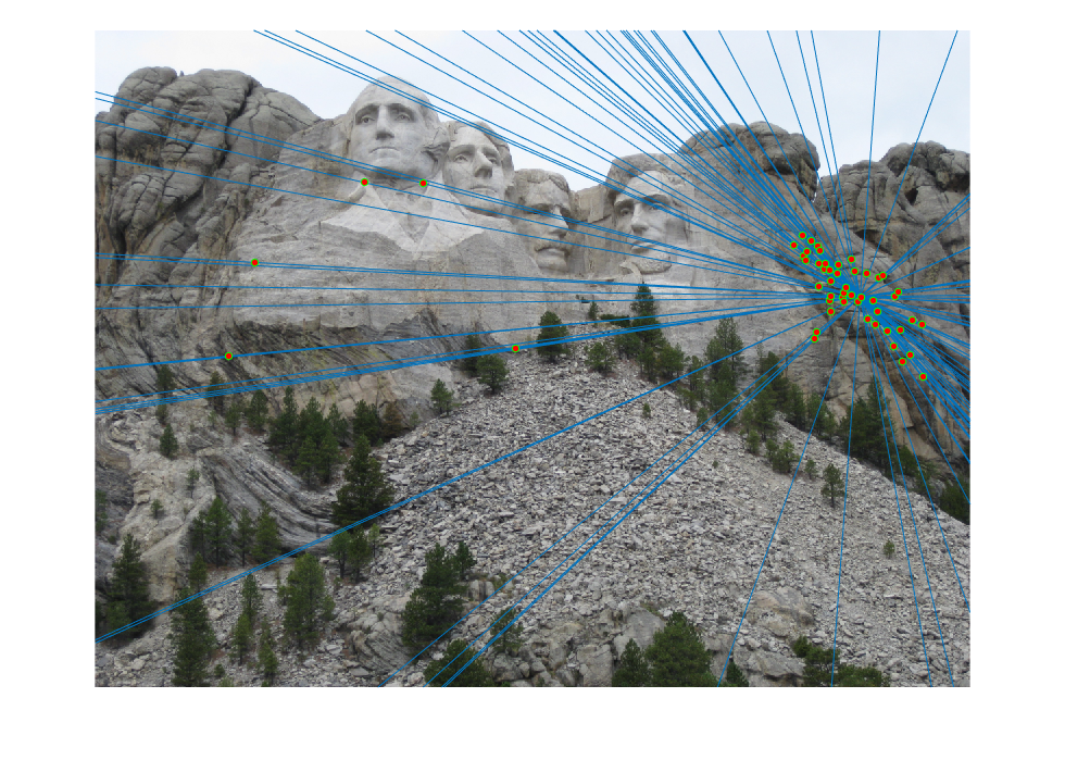
The improved results are shown below: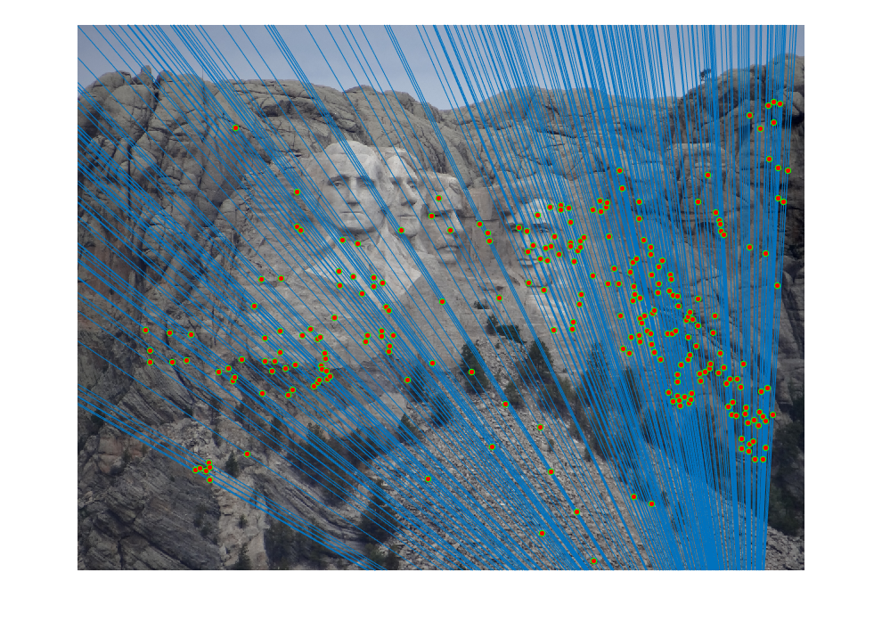