Project 3 / Camera Calibration and Fundamental Matrix Estimation with RANSAC
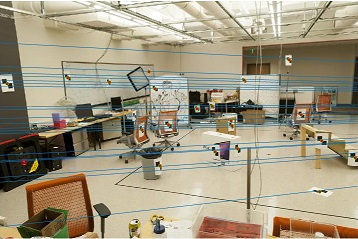
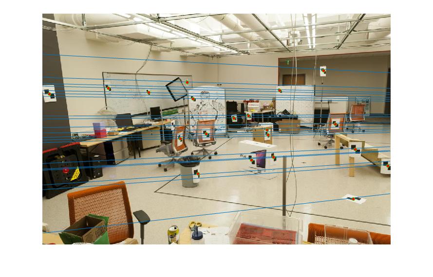
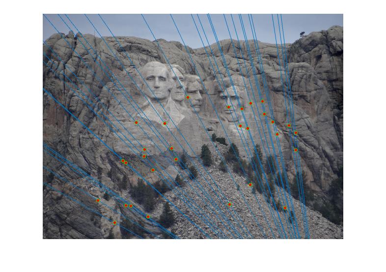
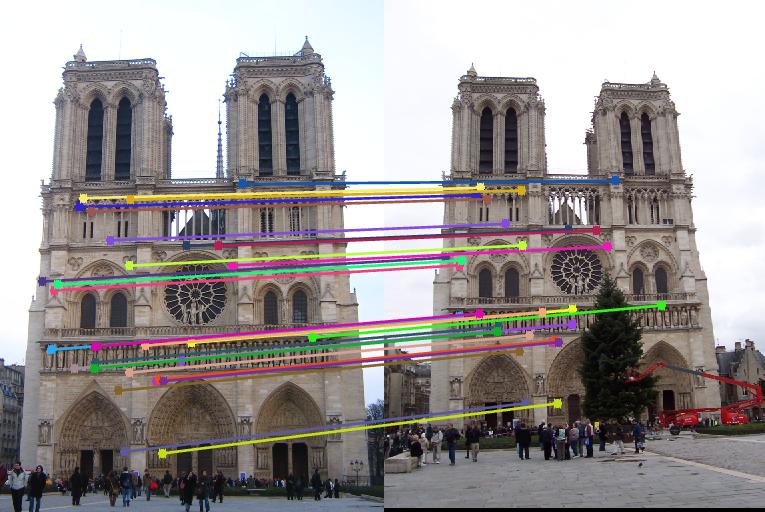
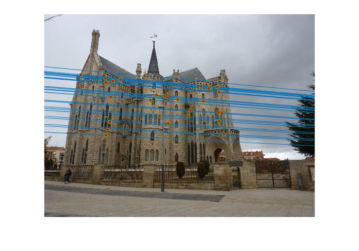
Example of an epipolar line convergence image.
Summary
Basic work:
- finding camera centers
- estimating the fundamental matrix for an image pair
- Ransac sampling method for detecting the best fundamental matrix
Extra work:
- adaptive iteration method based on unknown prior inlier rate
- normalizing the coordinates
Implementation details
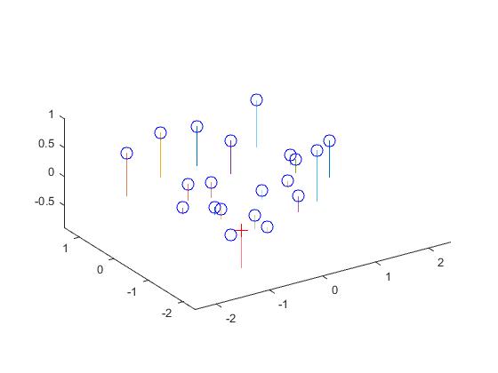
calculate_projection_matrix:
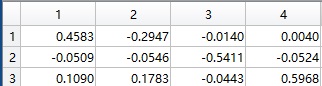
compute_camera_center:
Center is <-1.5127, -2.3517, 0.2826>. Total residue is <0.0445>
estimate_fundamental_matrix:
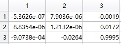
Sure there are multiple ways to construct the equation matrix for SVD. However, I believe my implementation is quite faster and neat by multipying the vectors in this orientation
for i = 1:size(Points_a,1)
    F = Homo_Points_a(i,:)' * Homo_Points_b(i,:);
    A(i,:) = F(:)';
end
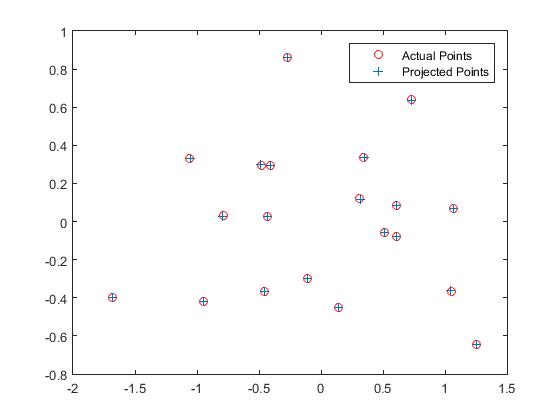
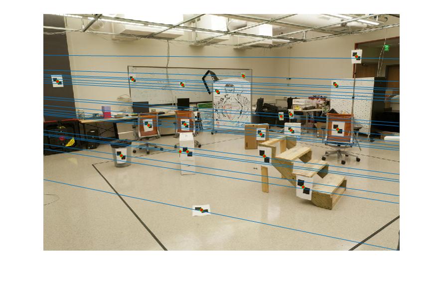
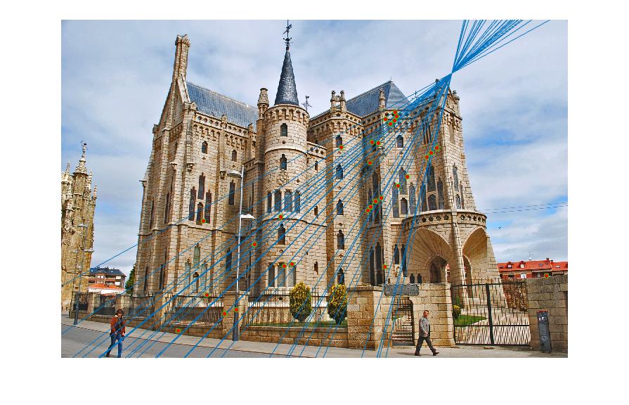
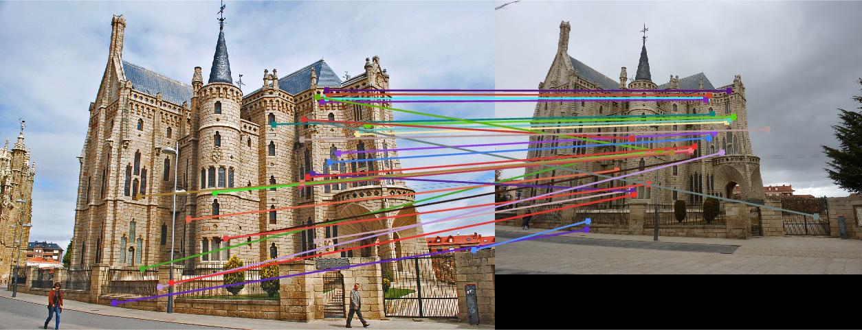
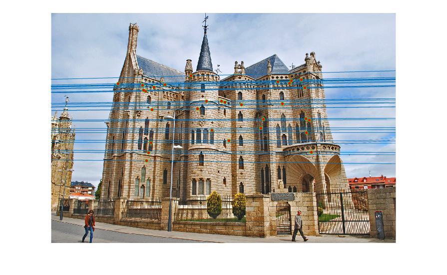
Here I also implemented coordinate normalization for graduate credit. Basically, I followed the instruction, calculated the mean and standard deviation of the two coordinate sets, constructed the transformation matrix, transform samples and then reverse the fundamental matrix. The resulting improvement was not so obvious on image pair 1 and 2, but became pretty good on image pair 3, as this pair is skewed severely.See Row 3 and 4 at Gallery section
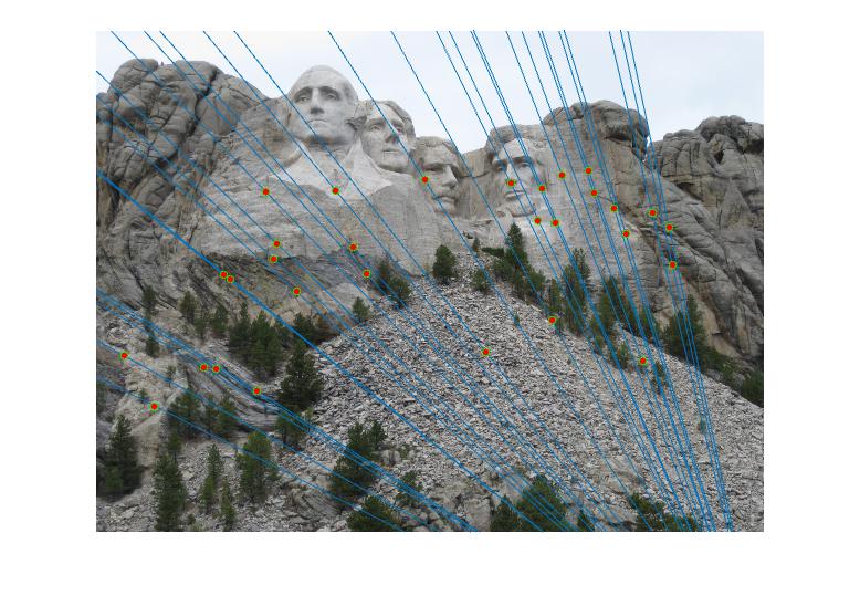
ransac_fundamental_matrix:
Here I used a faster way to multiply the pa' * F * pb ' for all points in vectorized form.
dummy = model_F * Homo_matches_a';
dummy = dummy';
sum(Homo_matches_b .* dummy, 2);
I also used adaptive iteration here. In this case, we can always get a model trained all with inliers even we do not know rate of inliers. Basically, each time I found a better inlier rate, I will re-compute the maximum number of iteration needed.In practice, when the confidence is high, say 99%, and tolerance is small, say 0.01, the maximum iteration number is generally 100000 for the first image pair. However, if tolerance is bigger, say 0.03, the iteration number would decrease to 10000
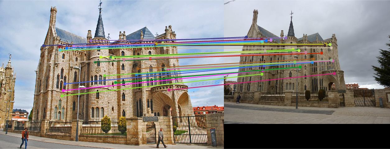
Gallery
|
|
|

|
|