Project 3: Camera Calibration and Fundamental Matrix Estimation with RANSAC
Part 1: Estimating the Projection Matrix and Camera Center
The first part of this project is calculating the camera projection matrix and then using it to find the camera center. The goal is to compute the matrix that goes from world 3D coordinates to 2D image coordinates. The way that I solved for the projection matrix was setting up a system of equations using the corresponding 2D and 3D points. Once I constructed the matrix representing the system of equations, I used Singular Value Decomposition to solve for the values of our M projection matrix. I was able to confirm my results by computing the residual and making sure it was small. Below is the code accomplishing calculating the projection matrix:
function M = calculate_projection_matrix( Points_2D, Points_3D )
    % create the A matrix for SVD
    A = zeros(size(Points_2D, 1) * 2, 12);
    for i = 1:size(A, 1)
        if (mod(i, 2) == 0)
            A(i, :) = [Points_3D(round(i/2), 1) Points_3D(round(i/2), 2) Points_3D(round(i/2), 3)...
            1 0 0 0 0 Points_3D(round(i/2), 1)*-1*Points_2D(round(i/2), 1)...
            Points_3D(round(i/2), 2)*-1*Points_2D(round(i/2), 1)...
            Points_3D(round(i/2), 3)*-1*Points_2D(round(i/2), 1) -1*Points_2D(round(i/2), 1)];
        else
            A(i, :) = [0 0 0 0 Points_3D(round(i/2), 1) Points_3D(round(i/2), 2) Points_3D(round(i/2), 3)...
            1 Points_3D(round(i/2), 1)*-1*Points_2D(round(i/2), 2)...
            Points_3D(round(i/2), 2)*-1*Points_2D(round(i/2), 2)...
            Points_3D(round(i/2), 3)*-1*Points_2D(round(i/2), 2) -1*Points_2D(round(i/2), 2)];
        end
    end

    [U, S, V] = svd(A);
    M = V(:,end);
    M = reshape(M, [], 3)';
end
After calculating the projection matrix, the final step for part 1 was to calculate the camera center. I did this by using what we talked about in class, taking the last column of our M matrix and using it with the Q (columns 1-3) of our M matrix to calculate our C camera center. The code to do this is below:
function [ Center ] = compute_camera_center( M )
    Q = M(1:3,1:3);
    M4 = M(:,4);
    Center = -1 * inv(Q) * M4;
end
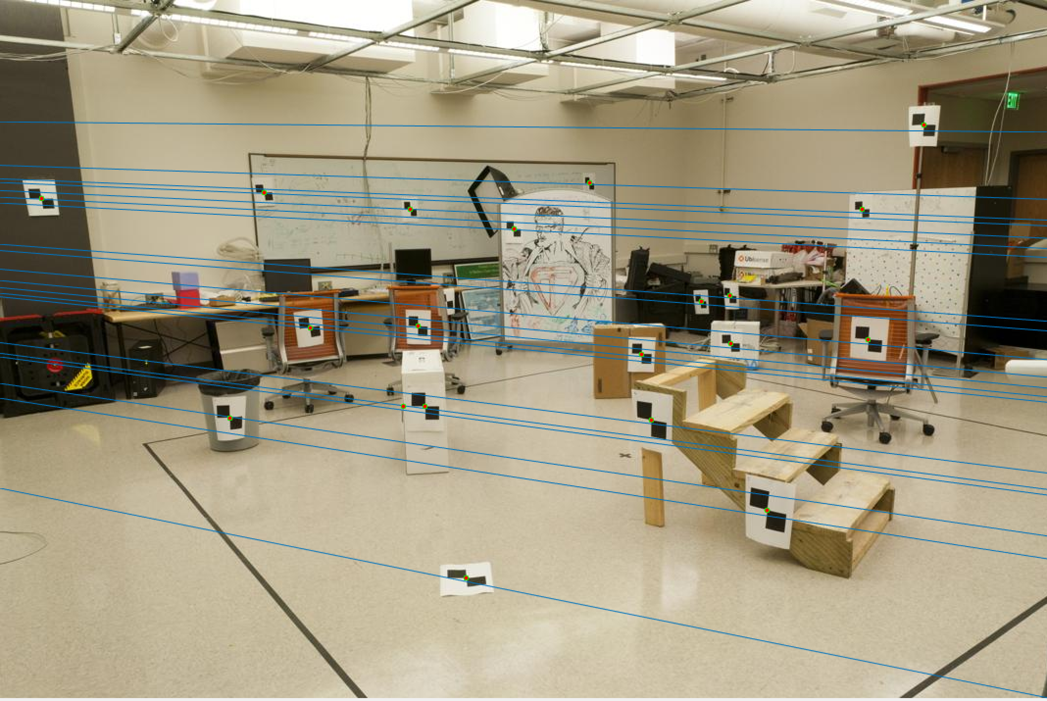
Finally, below are my results from running the first part of the project to confirm that my code performs as expected for the normalized points:
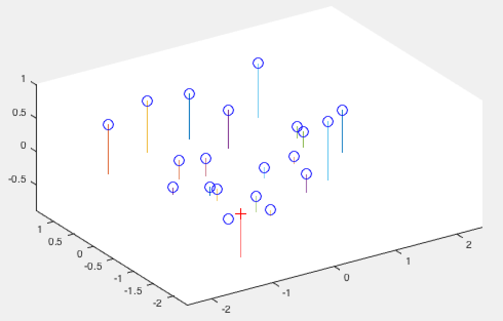
Normalized 3D View |
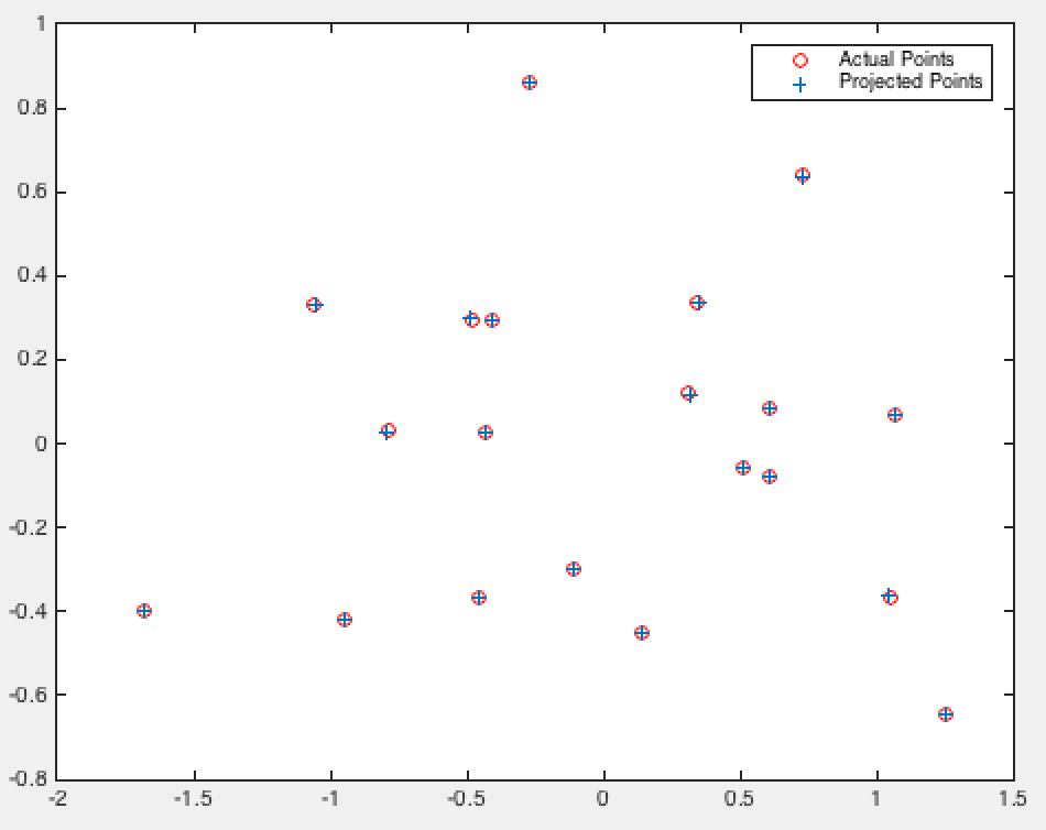
Normalized 2D View |
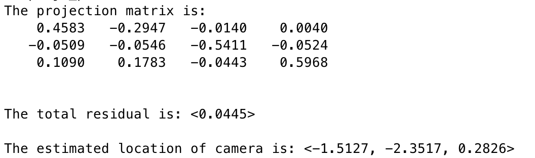
Normalized Matrix, Residual, Camera Center Results |
As we can see the camera center is only a rounding error off from the one mentioned in the project description, and our projection matrix is correct!
Part 2: Estimating Fundamental Matrix
For this portion of the project we estimate the fundamental matrix using the 8 point method. Here we do something similar to our first part, however, we set up a different matrix. We create a matrix representing our system of equations and then perform SVD and solve for f where Af = 0. Finally, we resolve det(F) = 0 using SVD once again, finally creating our F fundamental matrix. The code to accomplish this is below:
function [ F_matrix ] = estimate_fundamental_matrix(Points_a,Points_b)
    A = zeros(size(Points_a, 1), 9);
    for i = 1:size(A, 1)
        A(i,:) = [Points_a(i, 1)*Points_b(i, 1) Points_a(i, 1)*Points_b(i, 2) Points_a(i, 1)...
        Points_a(i, 2)*Points_b(i, 1) Points_a(i, 2)*Points_b(i, 2) Points_a(i, 2)...
        Points_b(i, 1) Points_b(i, 2) 1];
    end

    [U, S, V] = svd(A);
    f = V(:,end);
    F = reshape(f, [3 3]);

    [U, S, V] = svd(F);
    S(3, 3) = 0;
    F_matrix = U * S * V';
end
Now let us observe the results on our base image pair (pic_a.jpg and pic_b.jpg).
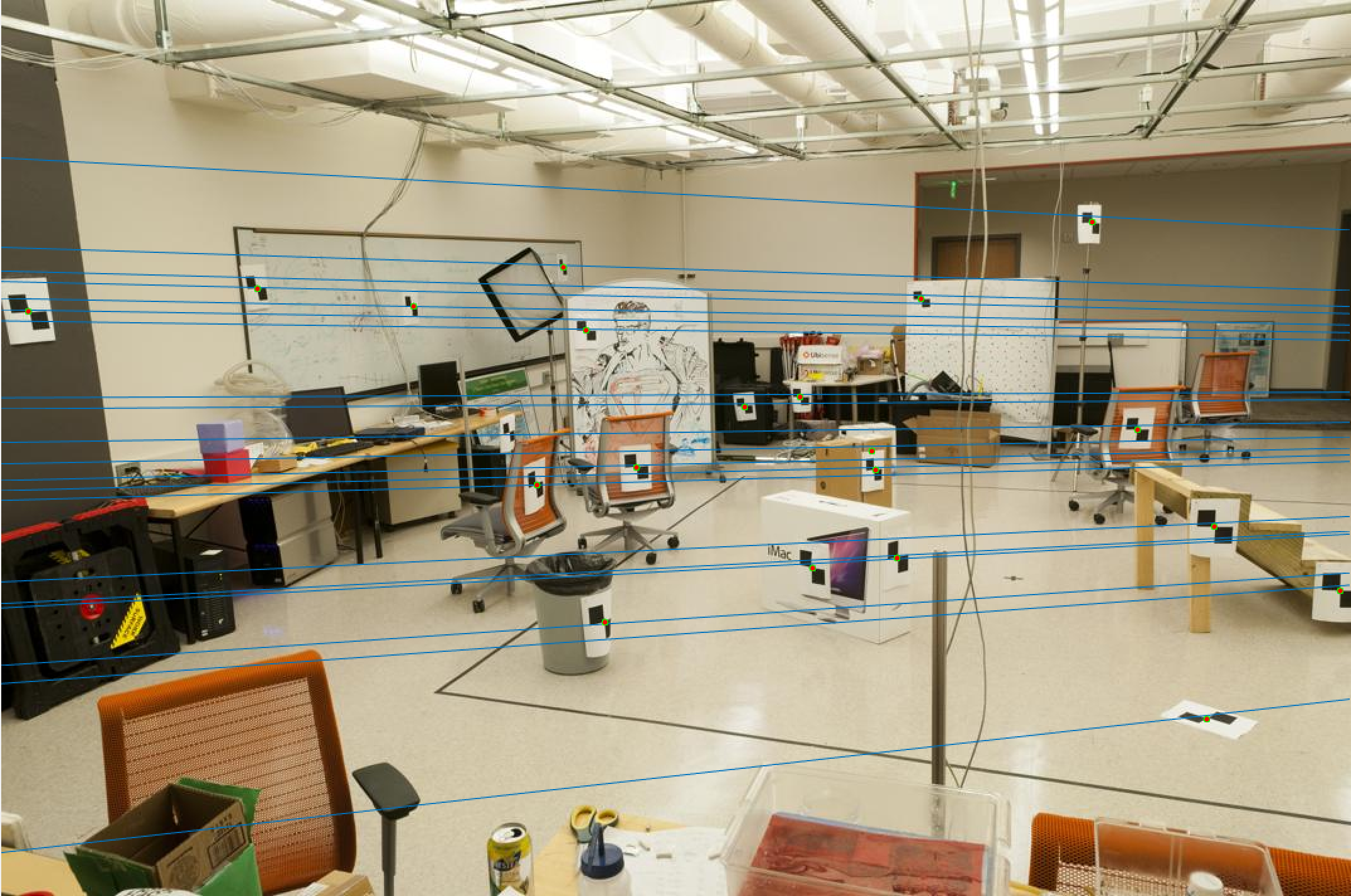
Pic 1 Epipolar Lines |
Pic 2 Epipolar Lines |
As we can see, these are exactly the results we want as our epipolar lines align quite well based on the human eye test.
Estimating Fundamental Matrix with Unreliable SIFT matches using RANSAC
The final part of this project focusing on computing the fundamental matrix without perfect point correspondences. Here we use RANSAC to compute the fundamental matrix frmo SIFT point correspondences. Due to outliers we can't use linear regression, so instead we use RANSAC. The jist of this algorithm is we pick 8 points (a number of points I chose) randomly, estimate the fundamental matrix, and determine how well it performs by counting inliers and outliers where an inlier is defined as a point that maintains the properties of our Fundamental Matrix that we know to be true based on some threshold which we define (in this case after trial and error I setted on a threshold of 0.02). We perform this for a reasonable number of iterations (there is a good way to estimate how many iterations are necessary but trial and error showed me that using 2000-4000 iterations was enough to produce good resutls). Finally we return the best fundamental matrix based on the number of points we identified as inliers. Know that the property we speak of with respect to the fundamental matrix is one that says taking point B in homogenous coordinates times F times point A in homogenous coordinates should give us a value of 0. By defining a threshold of 0.02 we are saying that any absolute value below 0.02 is close enough to be considered an inlier, helping to validate our estimated fundamental matrix. The code to accomplish this is shown below:
function [ Best_Fmatrix, inliers_a, inliers_b] = ransac_fundamental_matrix(matches_a, matches_b)
    best_num_inliers = 0;
    inliers_indicies = [];
    for i = 1:4000
        % randomly choose 8 points
        y = randsample(size(matches_a, 1), 8);
        % compute F given these 8 points
        f_matrix_est = estimate_fundamental_matrix(matches_a(y, :), matches_b(y, :));
        % check for all points how many are inliers and how many are outliers
        inliers = 0;
        temp_inliers = [];
        for j = 1:size(matches_a, 1)
            b_vec = [matches_b(j,:) 1];
            a_vec = [matches_a(j,:) 1];
            if (abs(b_vec * f_matrix_est * a_vec') < 0.02)
                inliers = inliers + 1;
                temp_inliers = [temp_inliers j];
            end
        end
        if inliers > best_num_inliers
            best_num_inliers = inliers;
            inliers_indicies = temp_inliers;
            best_matrix = f_matrix_est;
        end
        % keep best answer
    end

    Best_Fmatrix = best_matrix;
    inliers_a = matches_a(inliers_indicies, :);
    inliers_b = matches_b(inliers_indicies, :);
end
Examining Results for Various Images
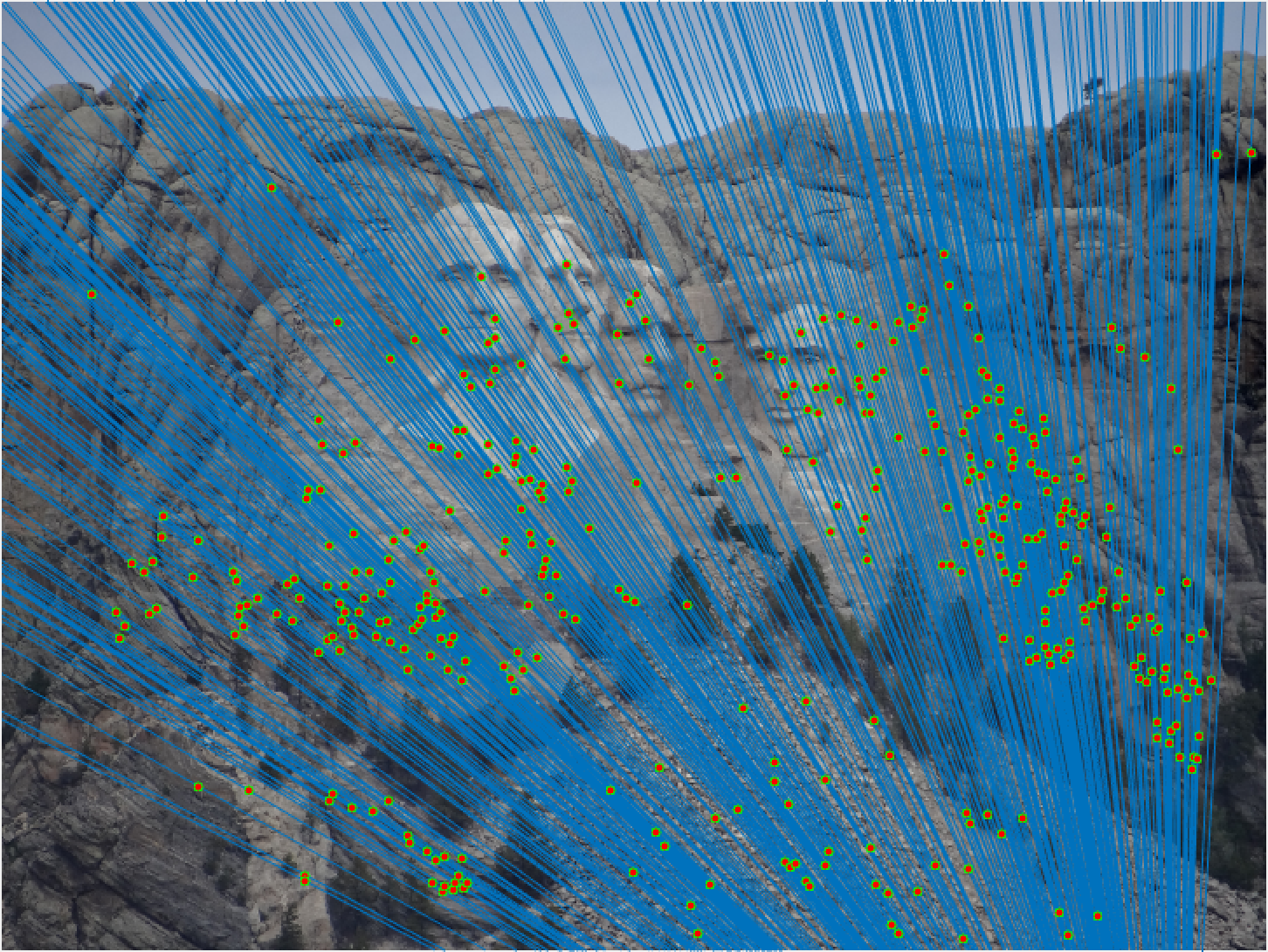
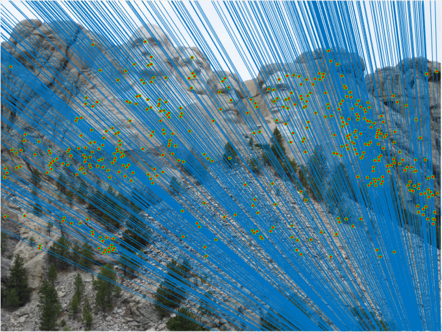
I found that the results produced were actually very good overall! The first image pair I show will show all of the inliers that we found with this RANSAC approach. In order to make it easier to view the inliers and the epipolar lines, for the first image pair and all subsequent I chose 30 random inliers to visualize in order to keep the images less clutterred.
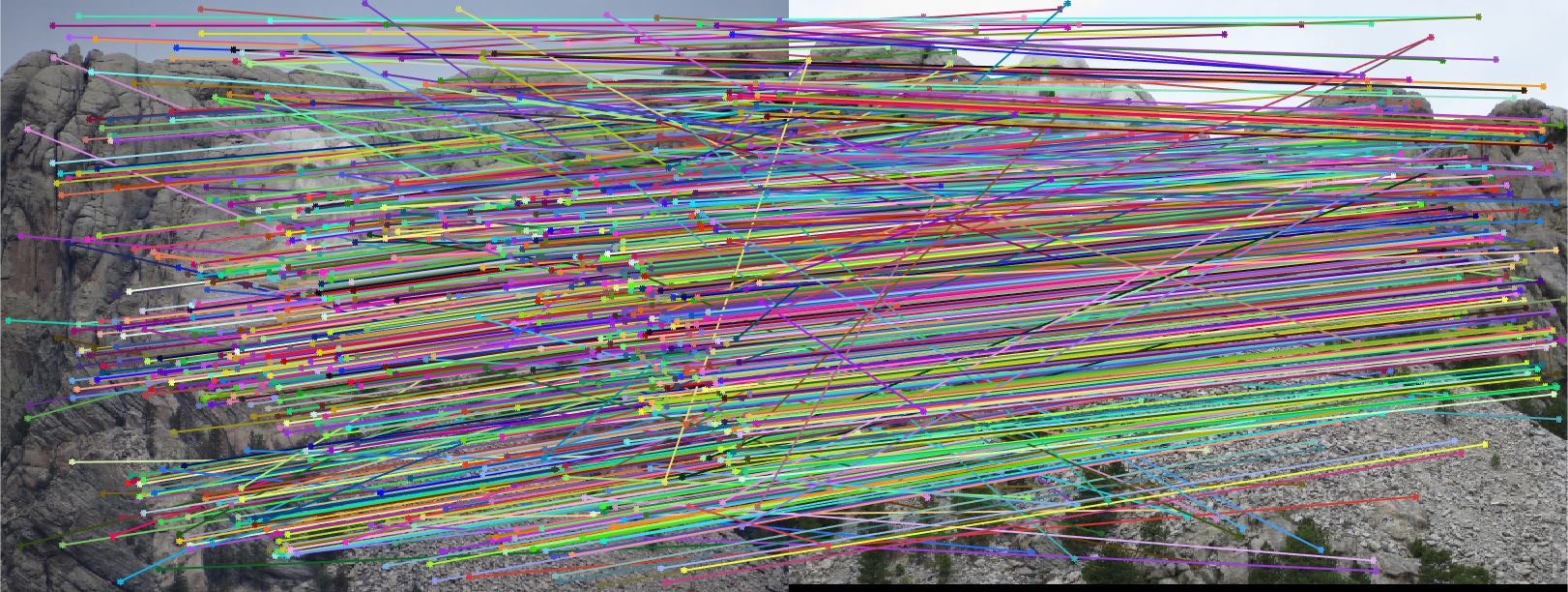
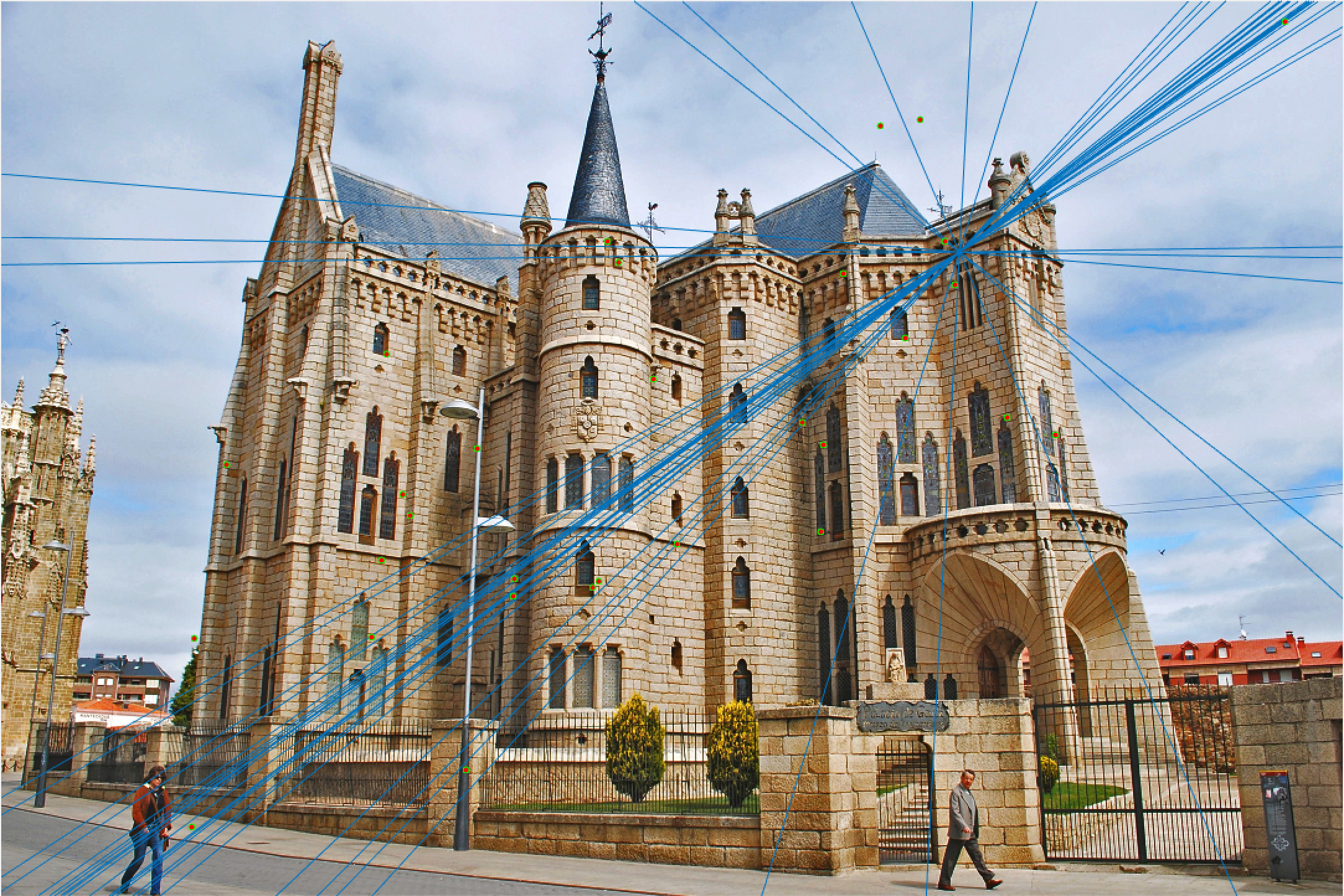
Mount Rushmore All SIFT Matches |
Mount Rushmore All Inliers |
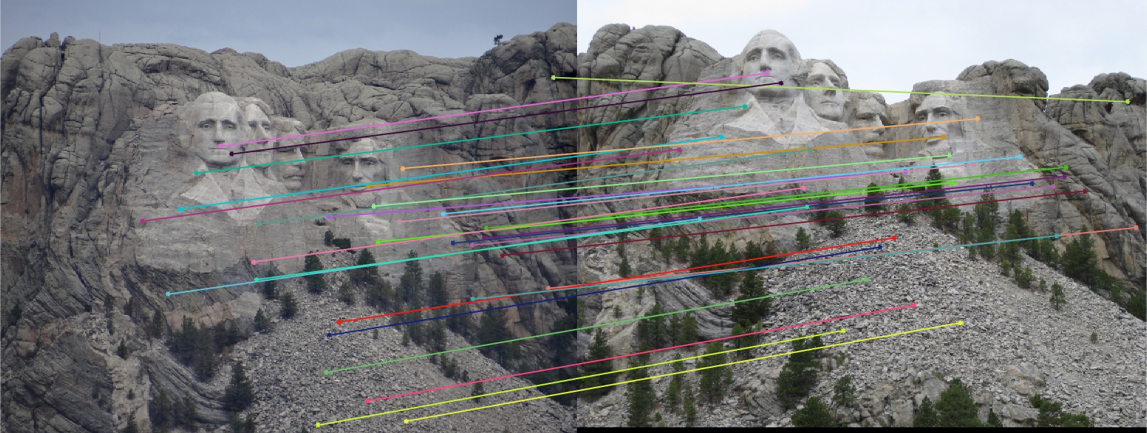
Mount Rushmore 30 Random Inliers |
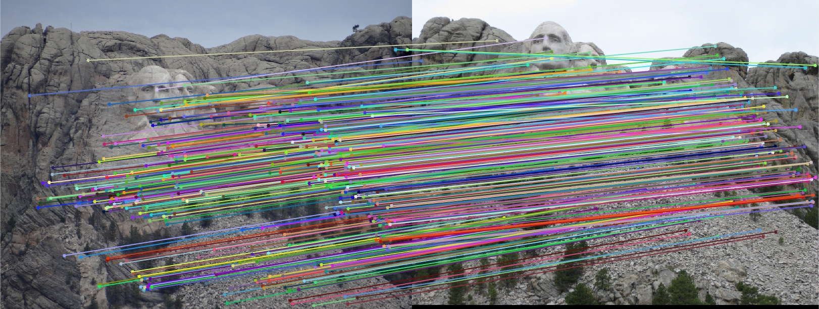
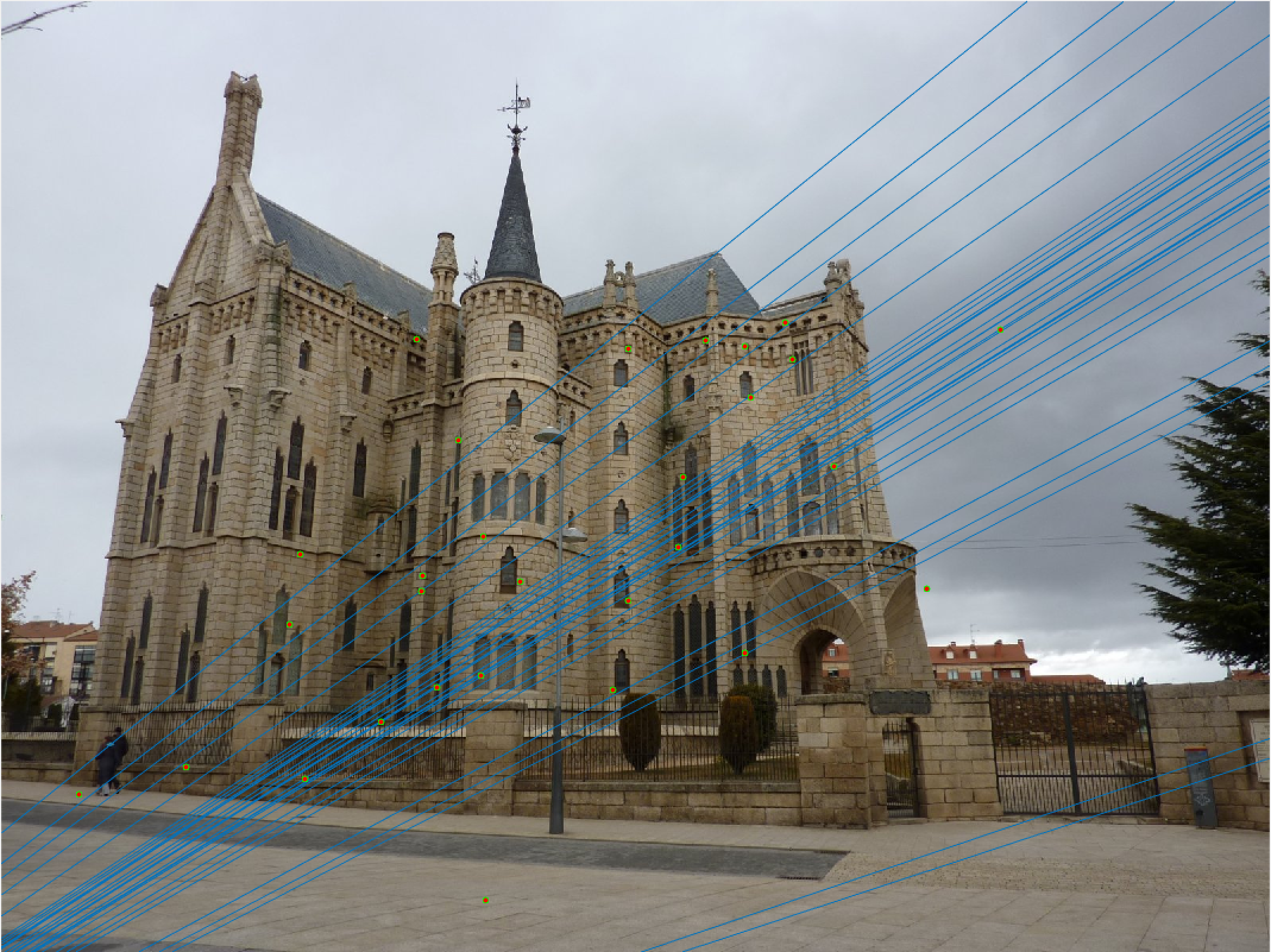
Mount Rushmore All Epipolar Lines |
Mount Rushmore All Epipolar Lines |
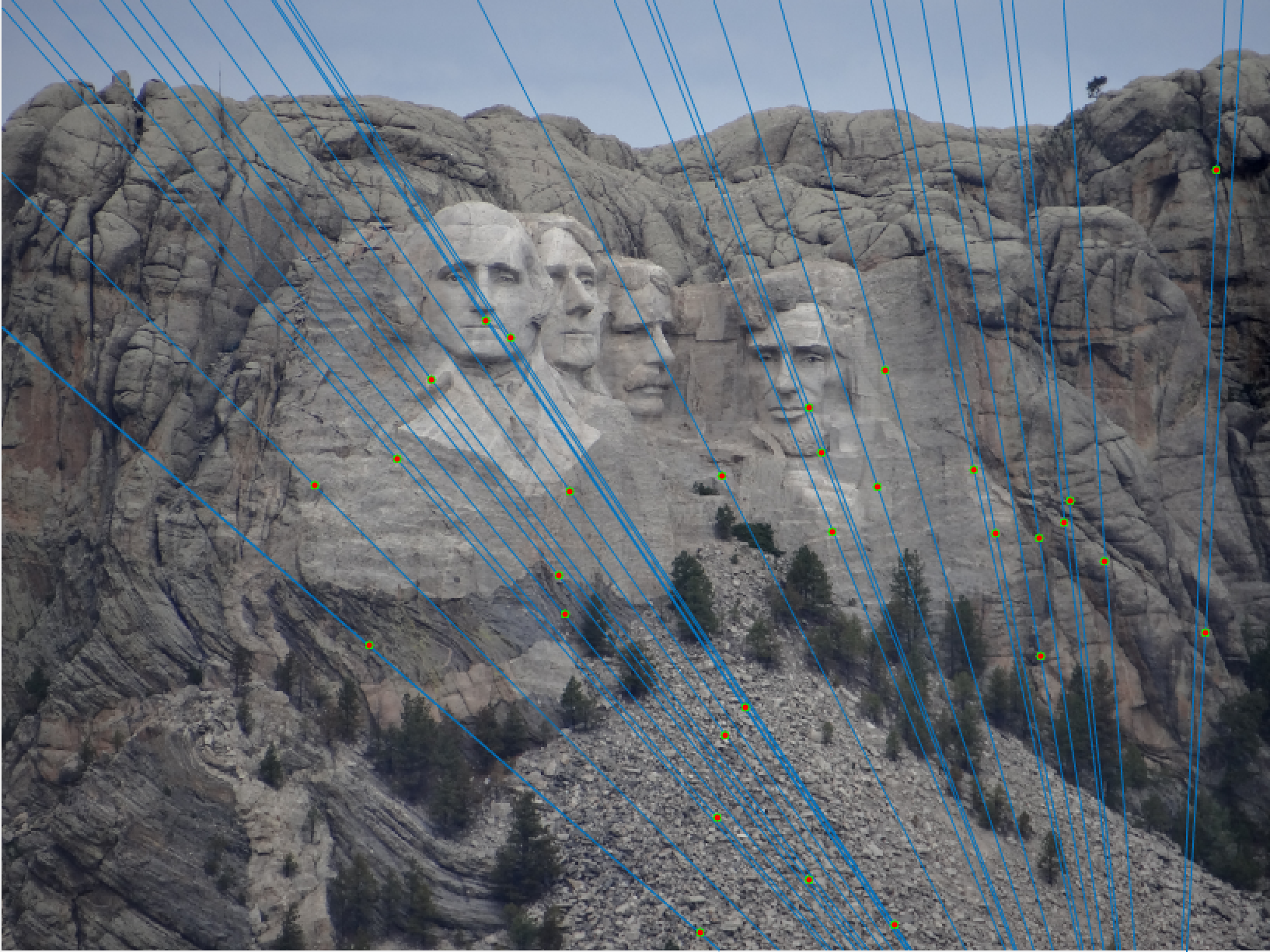
Mount Rushmore 30 Epipolar Lines |
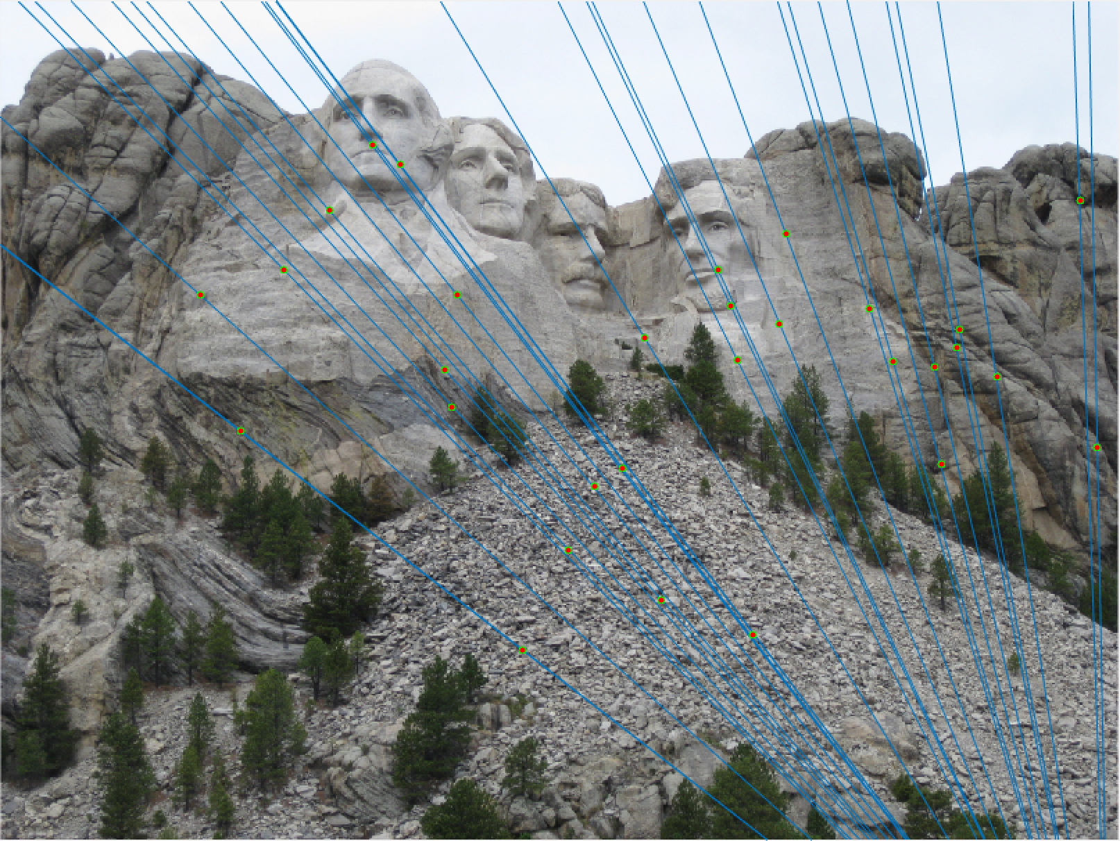
Mount Rushmore 30 Epipolar Lines |
We notice from both our epipolar lines and our feature matches that these are quite quite accurate! We can see this best when we look at a random 30 of the inliers we have identified. Furthermore, even with a low threshold we get quite a few inliers, which is good! We also notice how our epipolar lines in both images do a great job of going through the points we are looking at.
Now lets look at some other images to see if we continue to do a good job!
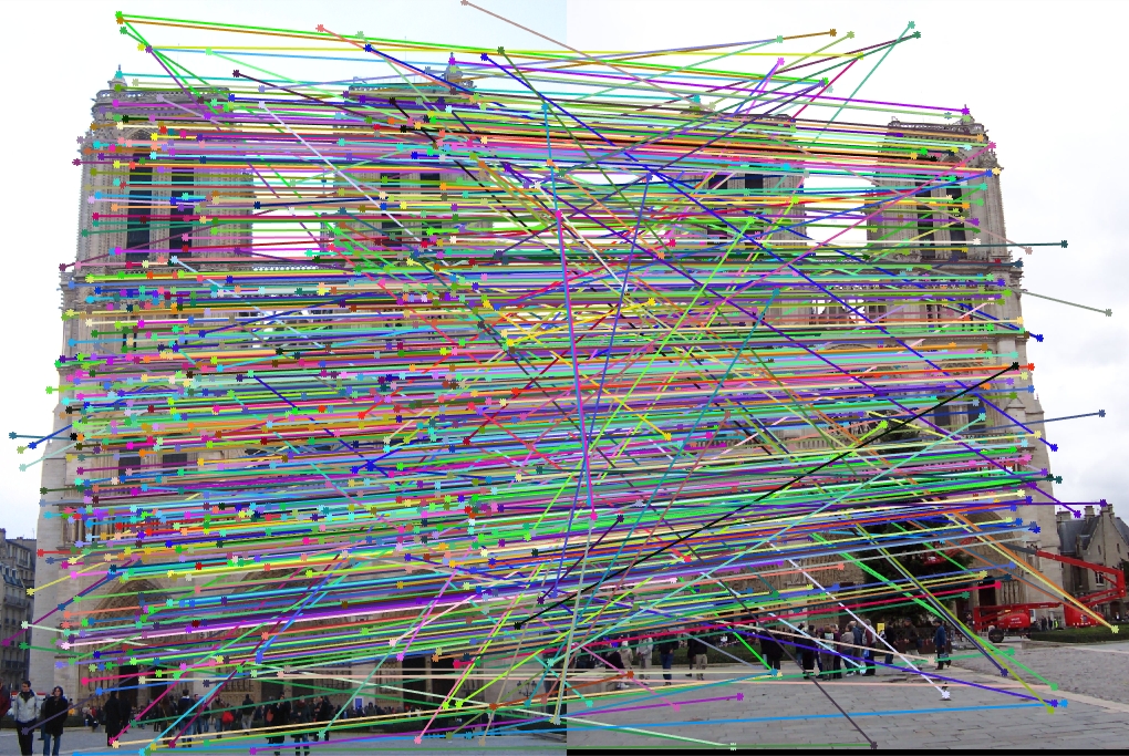
Notre Dame All SIFT Matches |
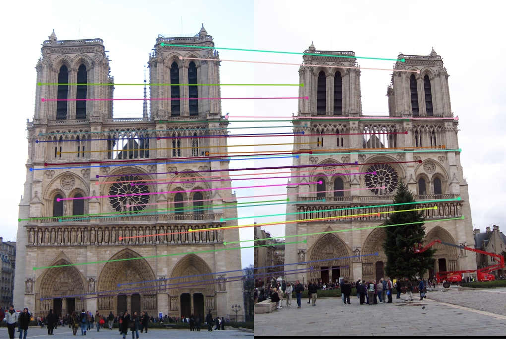
Notre Dame 30 Random Inliers |
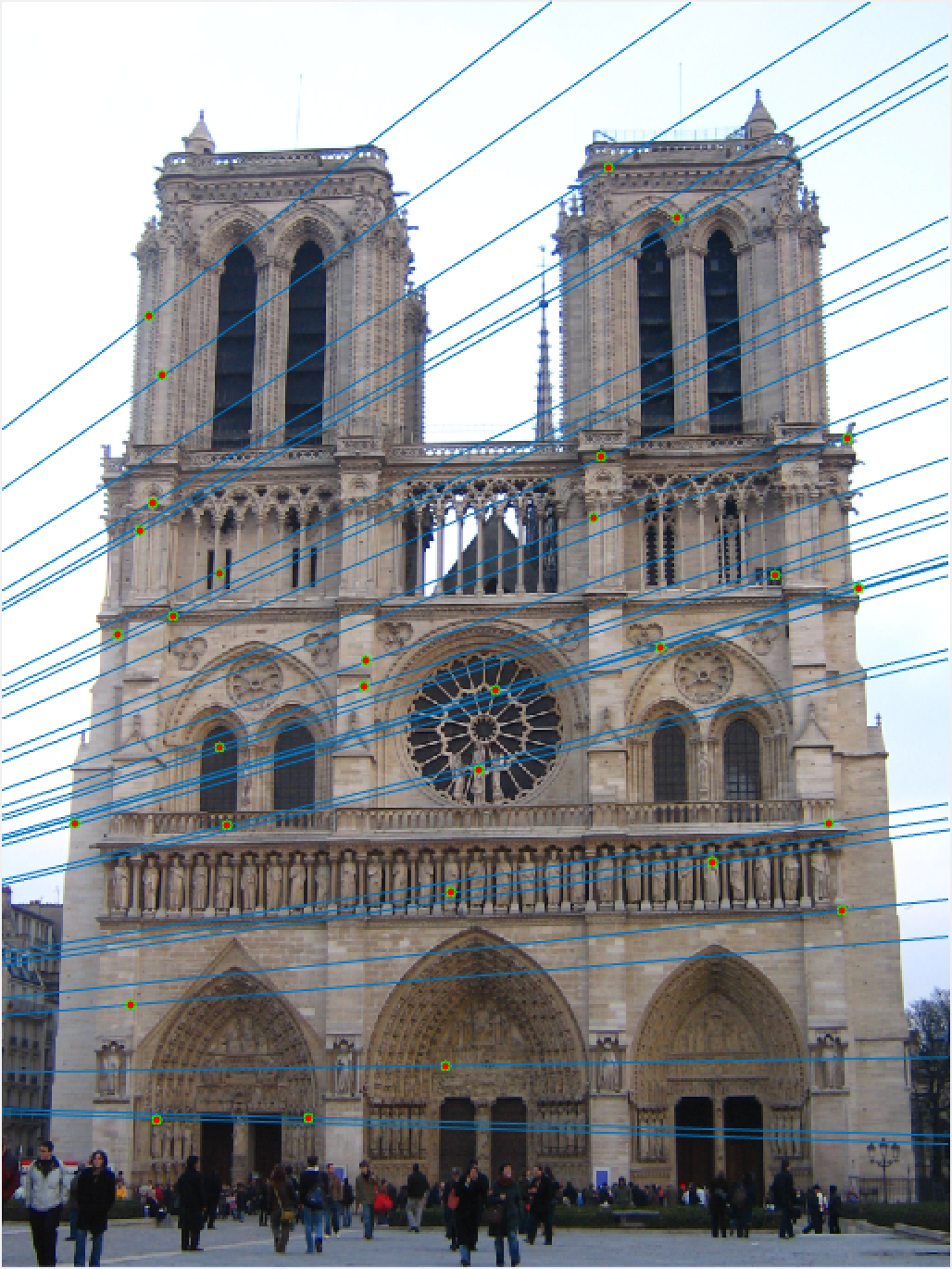
Notre Dame 30 Epipolar Lines |
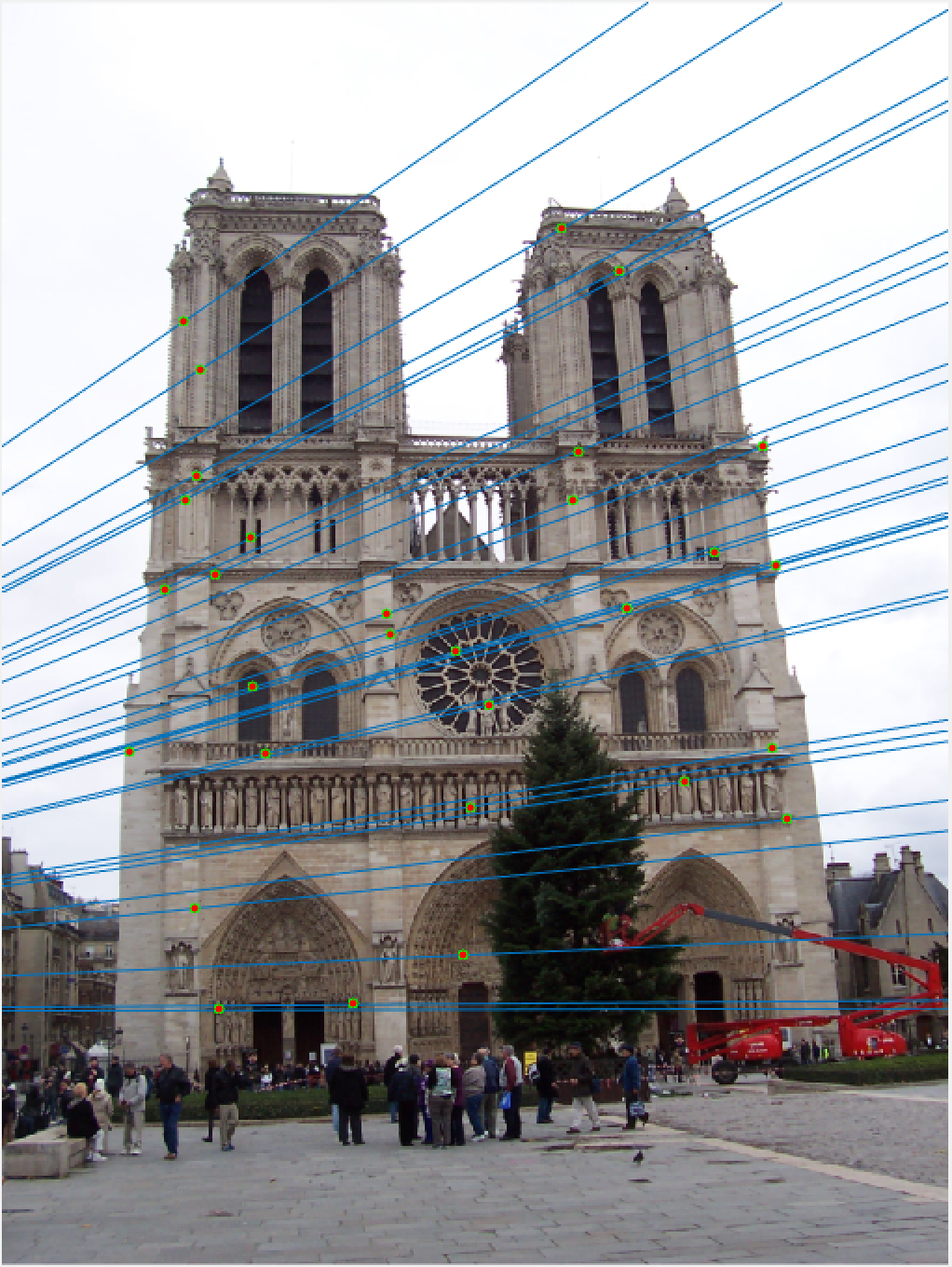
Notre Dame 30 Epipolar Lines |
Once again, our performance is quite good, this time on Notre Dame! As I mentioned, we are looking at a random 30 inliers, but these points have all been matched very well and our epipolar lines show that we have done a good job of estimating our fundamental matrix.
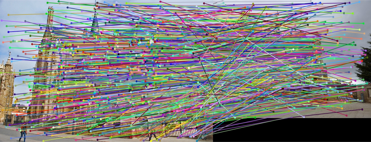
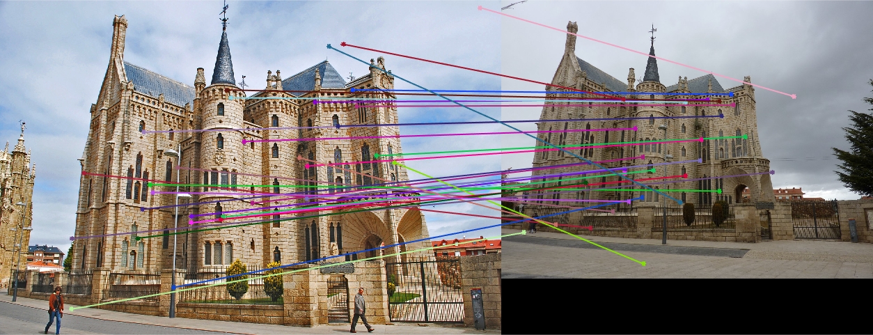
Episcopal Gaudi All SIFT Matches |
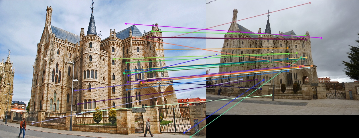
Episcopal Gaudi 30 Random Inliers |
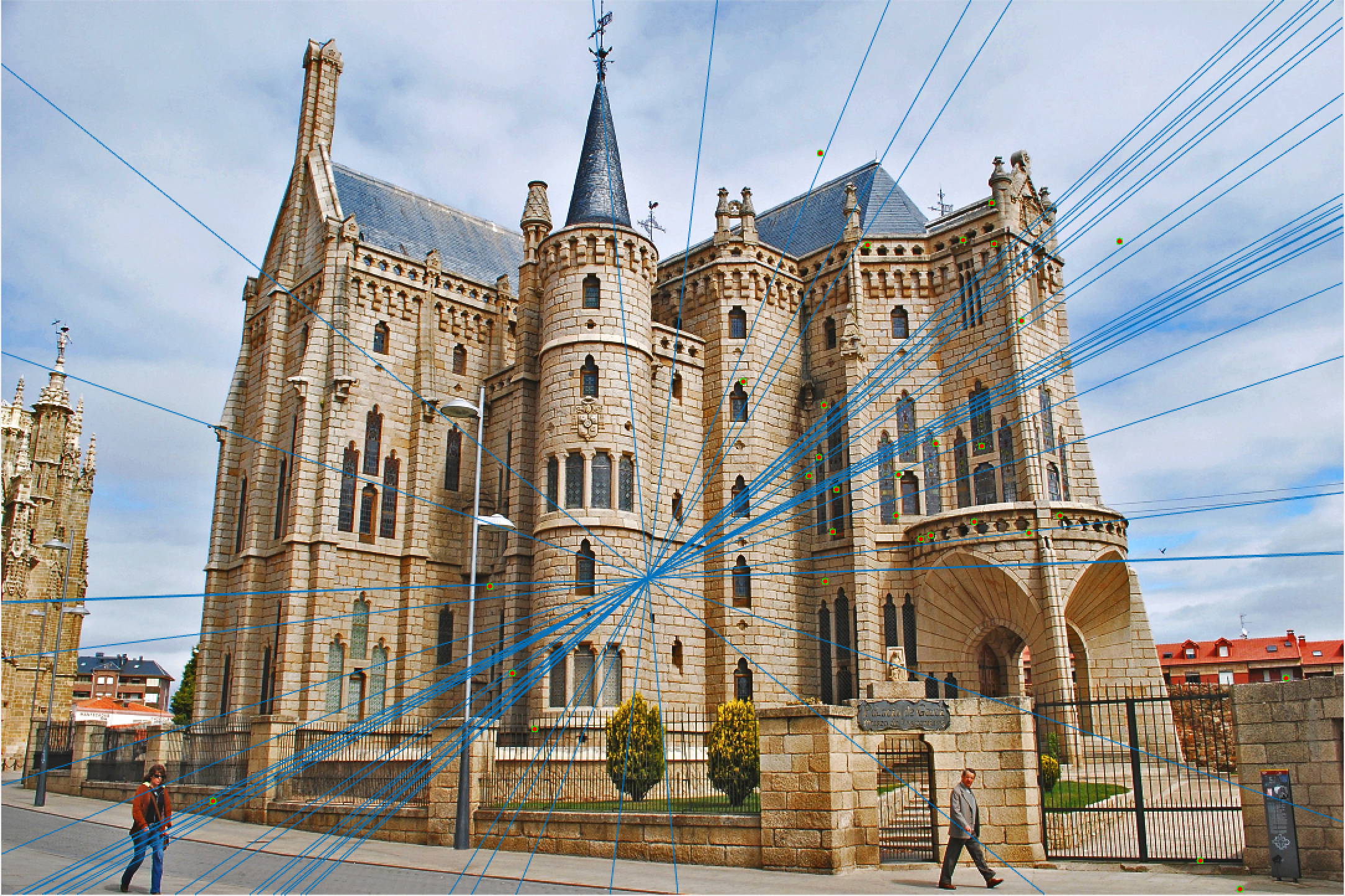
Episcopal Gaudi 30 Epipolar Lines |
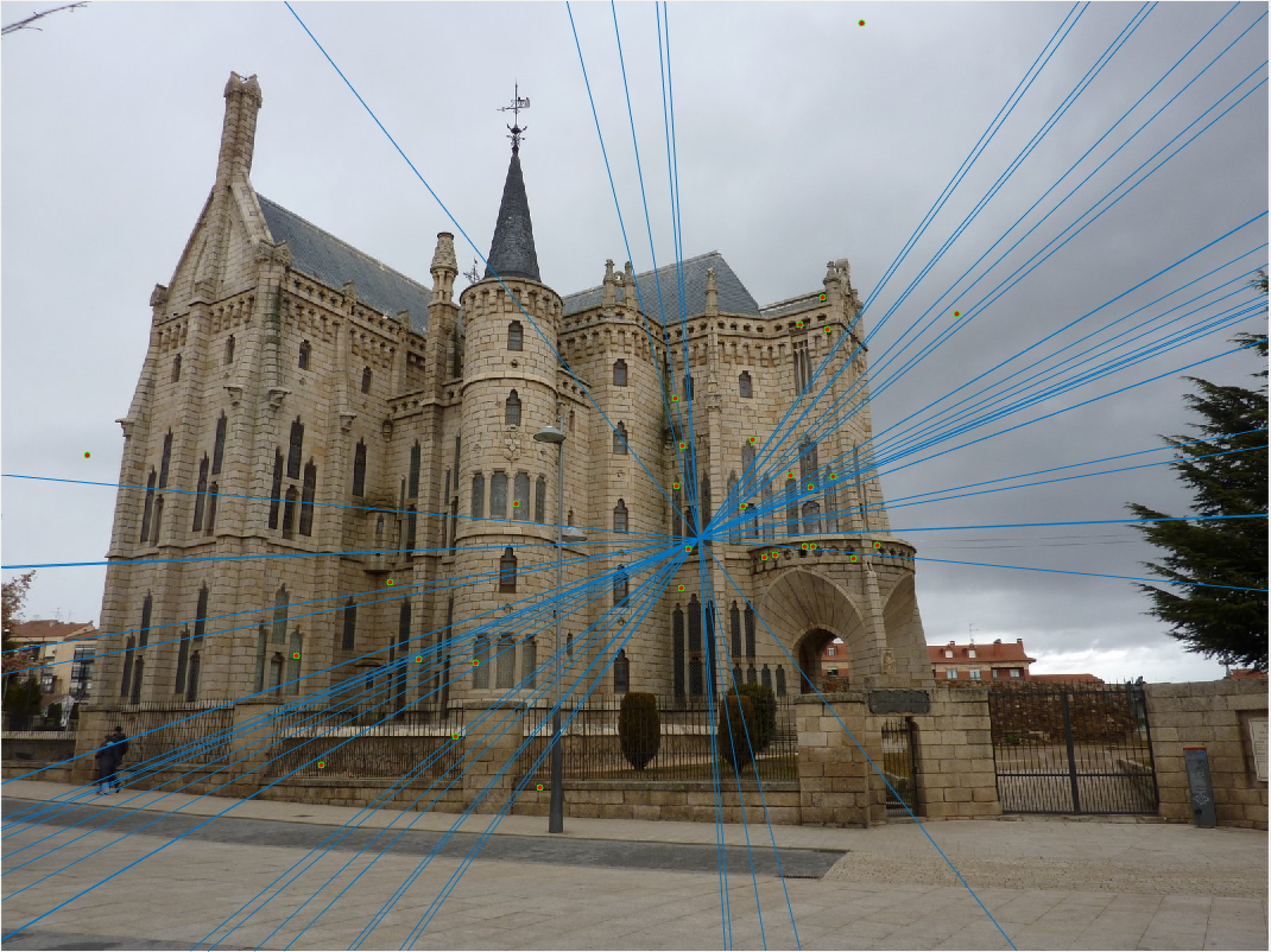
Episcopal Gaudi 30 Epipolar Lines |
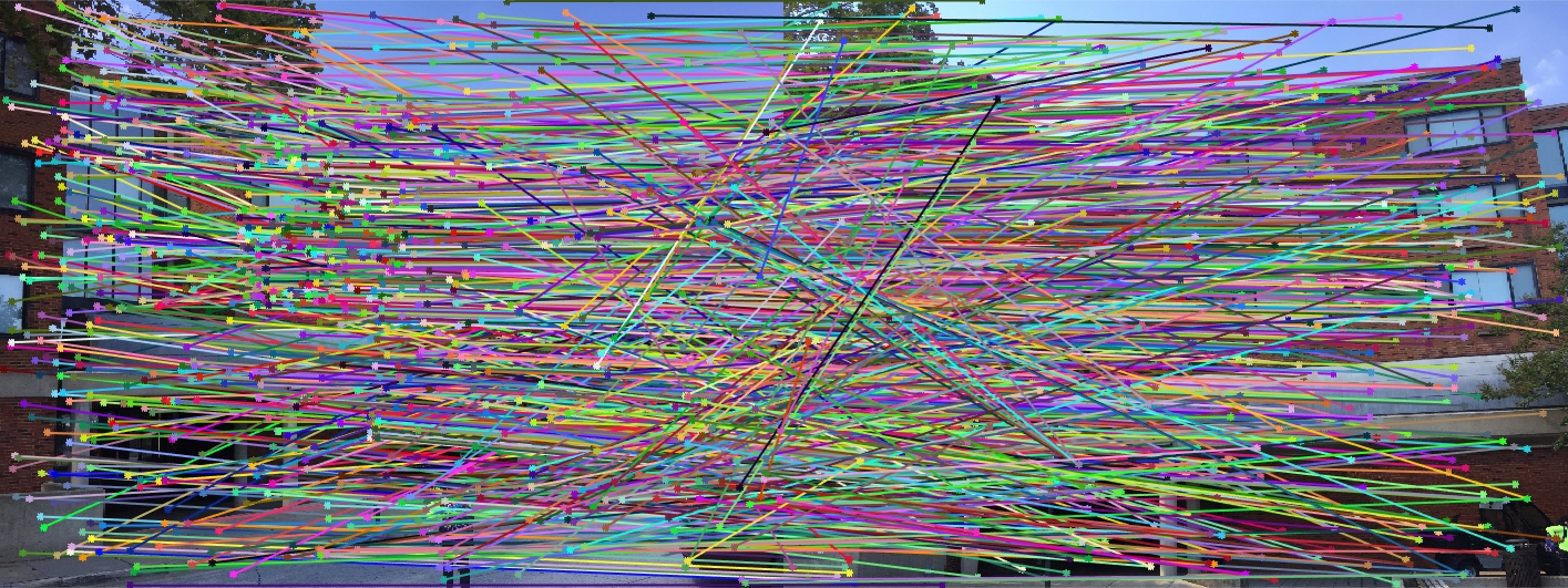
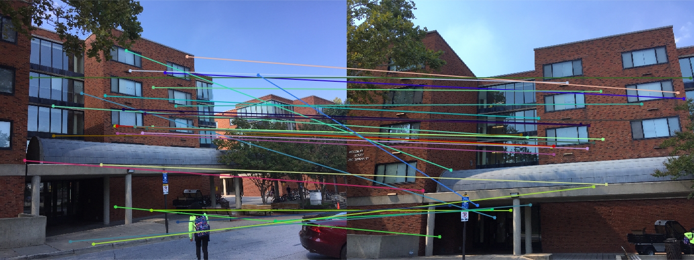
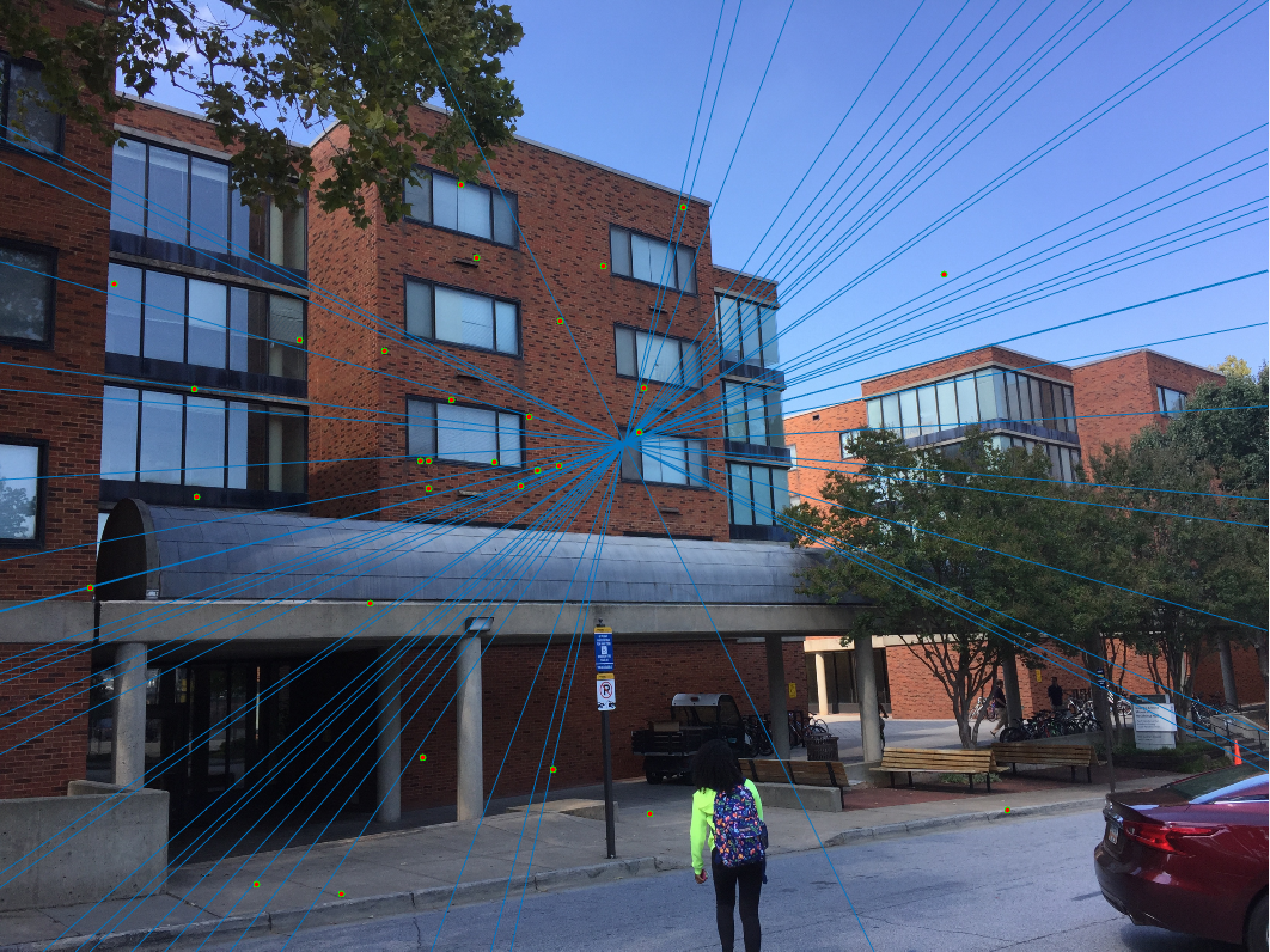
Woodruff Dorm All SIFT Matches |
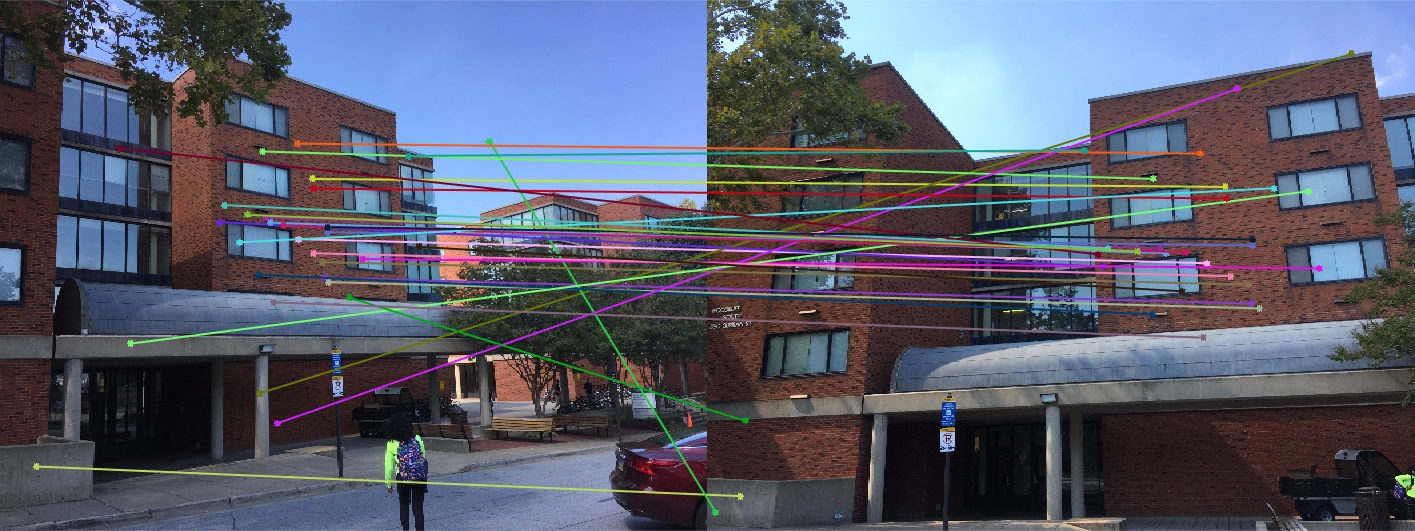
Woodruff Dorm 30 Random Inliers |
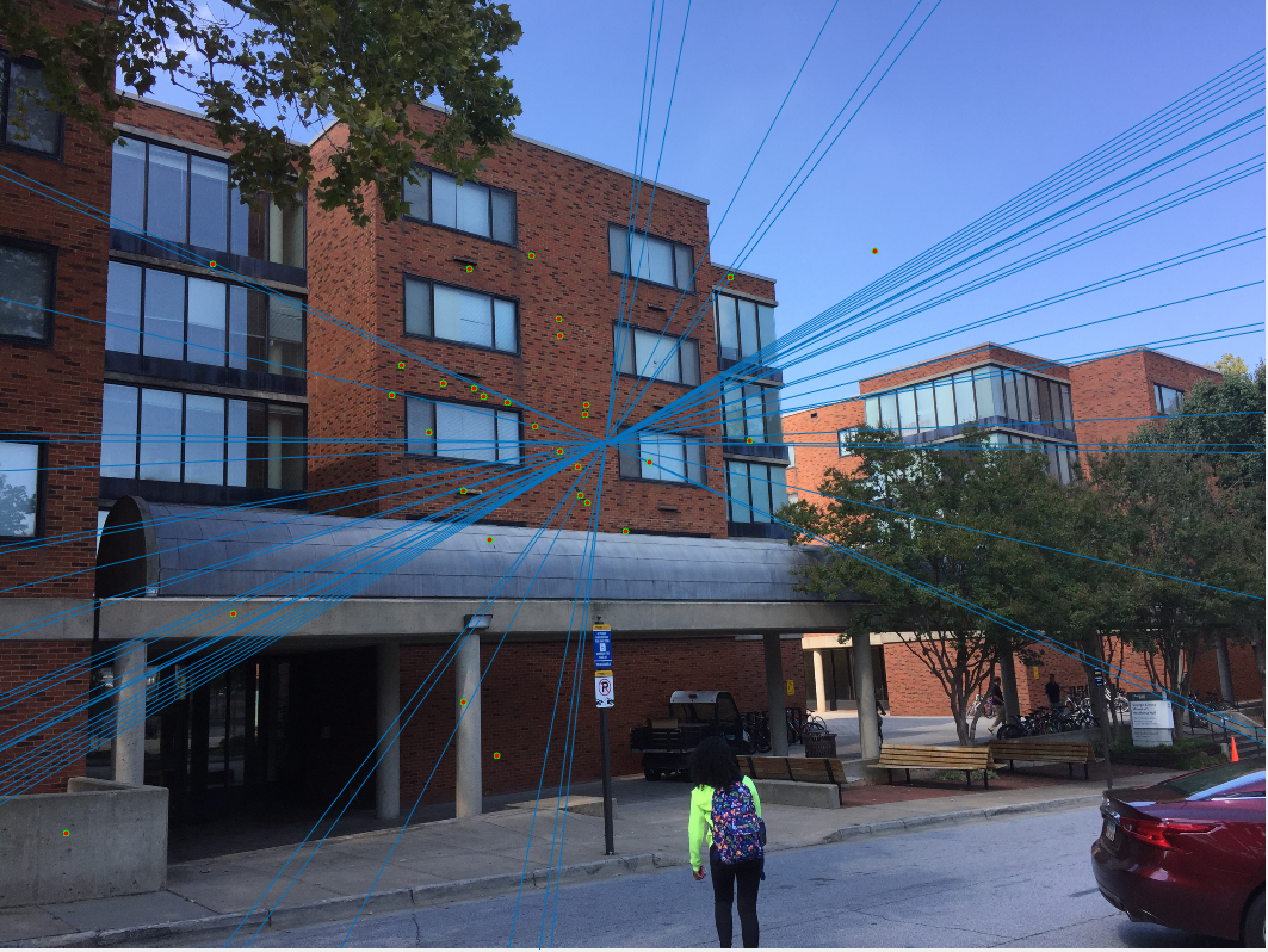
Woodruff Dorm 30 Epipolar Lines |
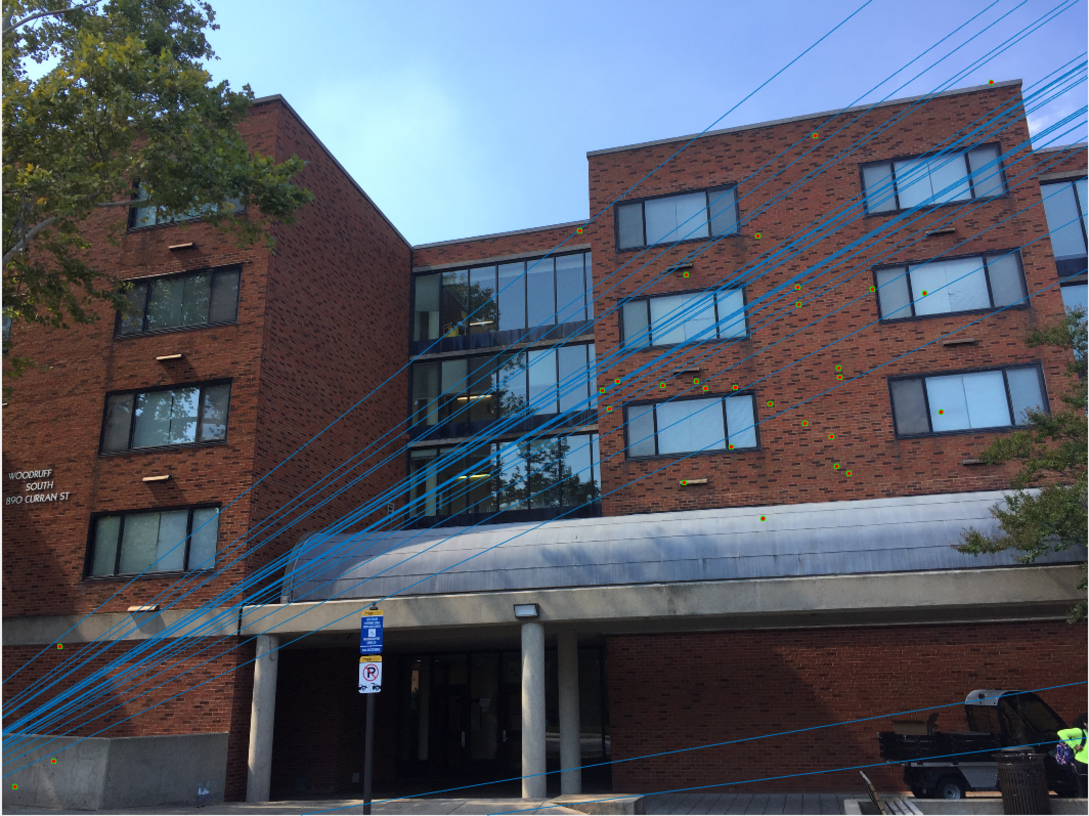
Woodruff Dorm 30 Epipolar Lines |
Here we see that for Episcopal Gaudi and Woodruff Dorm our results aren't quite as good as for our first two images. The epipolar lines still aren't too bad and some of the points actually match quite well (for instance near the central areas of the Woodruff Dorm building). This could likely be improved through normalization!
Extra Credit
I completed the extra credit for this project to improve my fundamental matrix estimation! I did this by creating transform matricies for our points and using them to normalize our points, compute our fundamental matrix, and then shift the fundamental matrix back into the original coordinates. The code I edited is in part 2 and is shown below:
% Create the T matrices for normalization
% find all the means
points_a_mean_u = mean2(Points_a(:,1));
points_a_mean_v = mean2(Points_a(:,2));
points_b_mean_u = mean2(Points_b(:,1));
points_b_mean_v = mean2(Points_b(:,2));

% repeat these means for easy standard deviation calculation
a_means_u = repmat(points_a_mean_u, size(Points_a,1), 1);
a_means_v = repmat(points_a_mean_v, size(Points_a,1), 1);
b_means_u = repmat(points_b_mean_u, size(Points_b,1), 1);
b_means_v = repmat(points_b_mean_v, size(Points_b,1), 1);

% find the standard deviations
sd_a_u = sqrt(sum((Points_a(:,1) - a_means_u).^2)/size(Points_a,1));
sd_a_v = sqrt(sum((Points_a(:,2) - a_means_v).^2)/size(Points_a,1));
sd_b_u = sqrt(sum((Points_b(:,1) - b_means_u).^2)/size(Points_b,1));
sd_b_v = sqrt(sum((Points_b(:,2) - b_means_v).^2)/size(Points_b,1));

% create T matrices!
Ta = [1/sd_a_u 0 points_a_mean_u/sd_a_u; 0 1/sd_a_v points_a_mean_v/sd_a_v; 0 0 1];
Tb = [1/sd_b_u 0 points_b_mean_u/sd_b_u; 0 1/sd_b_v points_b_mean_v/sd_b_v; 0 0 1];

% Transpose a and b points using these matrices
homog_a = [Points_a ones(size(Points_a,1), 1)]';
homog_b = [Points_b ones(size(Points_b,1), 1)]';
temp_a = Ta * homog_a;
temp_b = Tb * homog_b;
Points_a = [temp_a(1:2,:)'];
Points_b = [temp_b(1:2,:)'];

%% NORMAL CODE AS DESCRIBED IN PART 2

% change back F matrix to original coordinates
F_matrix = Tb'*F_matrix*Ta;
Below are the results for 30 random points for both episcopal gaudi and woodruff dorms, showing a small improvement from when we computed before normalizing our coordinates!
Episcopal Gaudi 30 Random Inliers Extra Credit |
Episcopal Gaudi 30 Epipolar Lines Extra Credit |
Episcopal Gaudi Epipolar Lines Extra Credit |
Woodruff Dorm 30 Random Inliers Extra Credit |
Woodruff Dorm 30 Epipolar Lines Extra Credit |
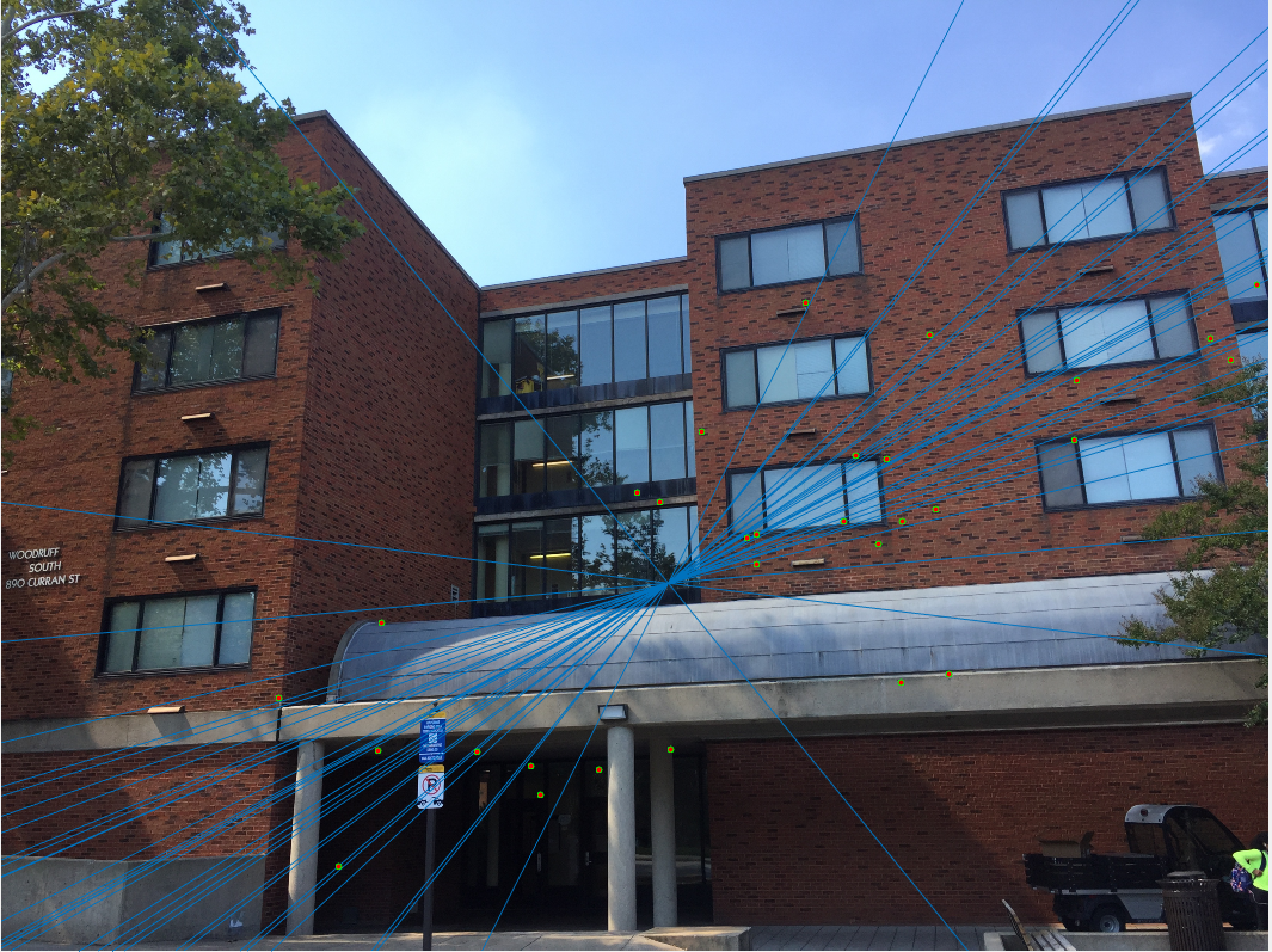
Woodruff Dorm 30 Epipolar Lines Extra Credit |
The improvement is most scene in episcopal gaudi, particularly from the epipolar lines! The woodruff dorm still caused some issues. With additional time I would try more and more iterations to see if it is possible with this method to get better lines and matches! It is worth noting that after making these code changes all of our other images still performed just as well as before, and we still got the same near-perfect results from part 2!