Jinsong Han

Camera Projection Matrix

The first part of the project was to calculate the projection matrix by using homogeneous coordinates. The projection matrix is what converts the real world 3D coordinates into 2D image coordinates (after being taken by a camera of some sort). This was solved by using linear regression to solve a systems of equations, which can be briefly described as the projection matrix (4 by 4 matrix) dot product with the real world 3D coordinates (4 by 1) results in the 2D image coordinates to some scale. When solving the linear regression, the degenerate (all zeros) case had to be avoided in order to actually find a useful solution. To resolve that issue, the last element of the projection matrix was fixed to 1, and the remaining coefficients were then calculated. Thus, the resulting projection matrix was scaled based on the hard-coded value of the last element in the projection matrix. The code for setting up the coefficients as part of the least squares regression (meaning A in the Ax=b equation) is shown below. Since the projection matrix (4 by 4) is being solved for (with one element set to 1), the least squares can be set up as A (coefficients of the respective M elements) times M (an 11 by 1 vector containing all the elements of the projection matrix minus one) which results in the 2D points that are being solved for.

% sets up the A matrix in the equation Ax=b to solve for least squares
for j = 0:points - 1
    % odd rows
    i = j + 1;
    odd = j * 2 + 1;
    A(odd, 1) = Points_3D(i, 1);
    A(odd, 2) = Points_3D(i, 2);
    A(odd, 3) = Points_3D(i, 3);
    A(odd, 4) = 1;
    A(odd, 9) = -Points_2D(i, 1) * Points_3D(i, 1);
    A(odd, 10) = -Points_2D(i, 1) * Points_3D(i, 2);
    A(odd, 11) = -Points_2D(i, 1) * Points_3D(i, 3);

    % even rows
    even = j * 2 + 2;
    A(even, 5) = Points_3D(i, 1);
    A(even, 6) = Points_3D(i, 2);
    A(even, 7) = Points_3D(i, 3);
    A(even, 8) = 1;
    A(even, 9) = -Points_2D(i, 2) * Points_3D(i, 1);
    A(even, 10) = -Points_2D(i, 2) * Points_3D(i, 2);
    A(even, 11) = -Points_2D(i, 2) * Points_3D(i, 3);
end

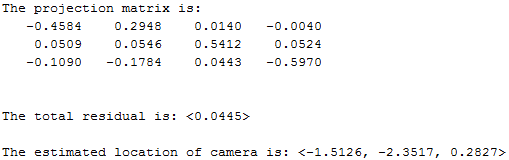
Now, from that projection matrix, the camera center in world coordinates was estimated. The projection matrix M can be split into a 3x3 matrix called Q and the final 3x1 vector that is called m4 (since it is the fourth column of the matrix). The camera center can then be calculated by doing the dot product between negative Q inverse and m4.

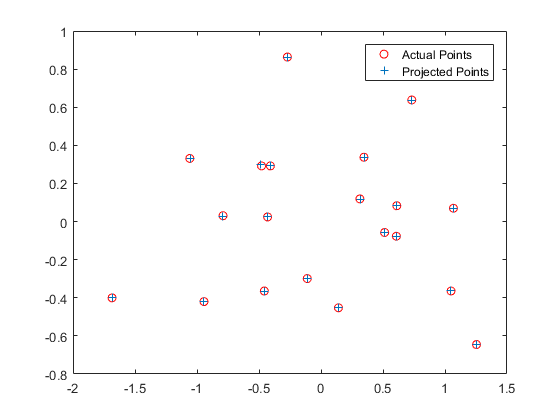
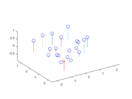
The estimated projection matrix from the given points and estimated camera location is shown below, including some visualizations.

Fundamental Matrix Estimation

The second part of the project was to calculate the fundamental matrix given a set of matched points between two images. The fundamental matrix is used to estimate the mapping of points in one images to lines (that correspond to the depth of the original image) in another image. These lines are called epipolar lines, and can ultimately be used to filter out incorrect matches (as matches originally calculated that do not fall on the calculated epipolar lines are likely to be incorrect).

An important property of the fundamental matrix is that the point on the second image as a 3x1 vector transposed (x_b') dot product with the fundamental matrix dot product with the corresponding point on the first image as a 3x1 vector (x_a) should yield 0. In other words, x_b' * F * x_a = 0. This is the case because x_b' * F gives us the resulting epipolar line for where the same point could appear in the other (a) image depending on depth. Finally, the result dot product with x_a should give 0, as the point should be on the calculated resulting line. Thus, a regression equation can be created and solved for given enough points to work with - in this case, 8 points are needed since the fundamental matrix (a 3x3 matrix) has at most 8 degrees of freedom (generally one or two elements are used for scale). The 8-point algorithm can then be used to solve for the fundamental matrix. However, the resulting estimate will be full rank. The fundamental matrix however must be a rank 2 matrix. This is because the fundamental matrix is essentially derived from the essential matrix, which is equal to the rotation matrix and the translation matrix as a cross product 3x3 matrix - where one of its columns is a linear combination of the other two columns, meaning that the translation matrix is rank 2. Therefore, the fundamental matrix must also be rank 2. To make the calculated fundamental matrix satisfy this property, the calculated fundamental matrix can be decomposed using singular value decomposition, resulting in U ΣV'. The smallest value in Σ can be set to zero and then multiplied back together to receive our final rank 2 fundamental matrix. The code for this is shown below.

% sets up the coefficient matrix to use in the 8-point algorithm
for i = 1:points
    A(i, 1) = Points_a(i, 1) * Points_b(i, 1);
    A(i, 2) = Points_a(i, 2) * Points_b(i, 1);
    A(i, 3) = Points_b(i, 1);
    A(i, 4) = Points_a(i, 1) * Points_b(i, 2);
    A(i, 5) = Points_a(i, 2) * Points_b(i, 2);
    A(i, 6) = Points_b(i, 2);
    A(i, 7) = Points_a(i, 1);
    A(i, 8) = Points_a(i, 2);
    A(i, 9) = 1;
end

% solve for f from Af=0 by using singular value decomposition
[U, S, V] = svd(A);
f = V(:, end);
F = reshape(f, [3 3]);
F = transpose(F);

% make F rank 2
[U, S, V] = svd(F);
if (S(1, 1) <= S(2, 2) && S(1, 1) <= S(3, 3))
    S(1, 1) = 0;
elseif (S(2, 2) <= S(1, 1) && S(2, 2) <= S(3, 3)) 
    S(2, 2) = 0;
else
    S(3, 3) = 0;
end
F_matrix = U * S * V';

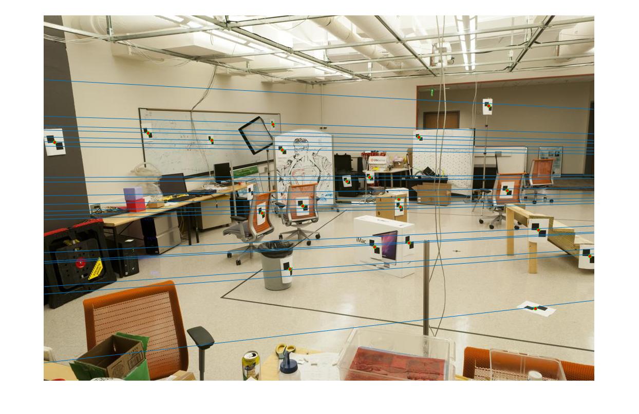
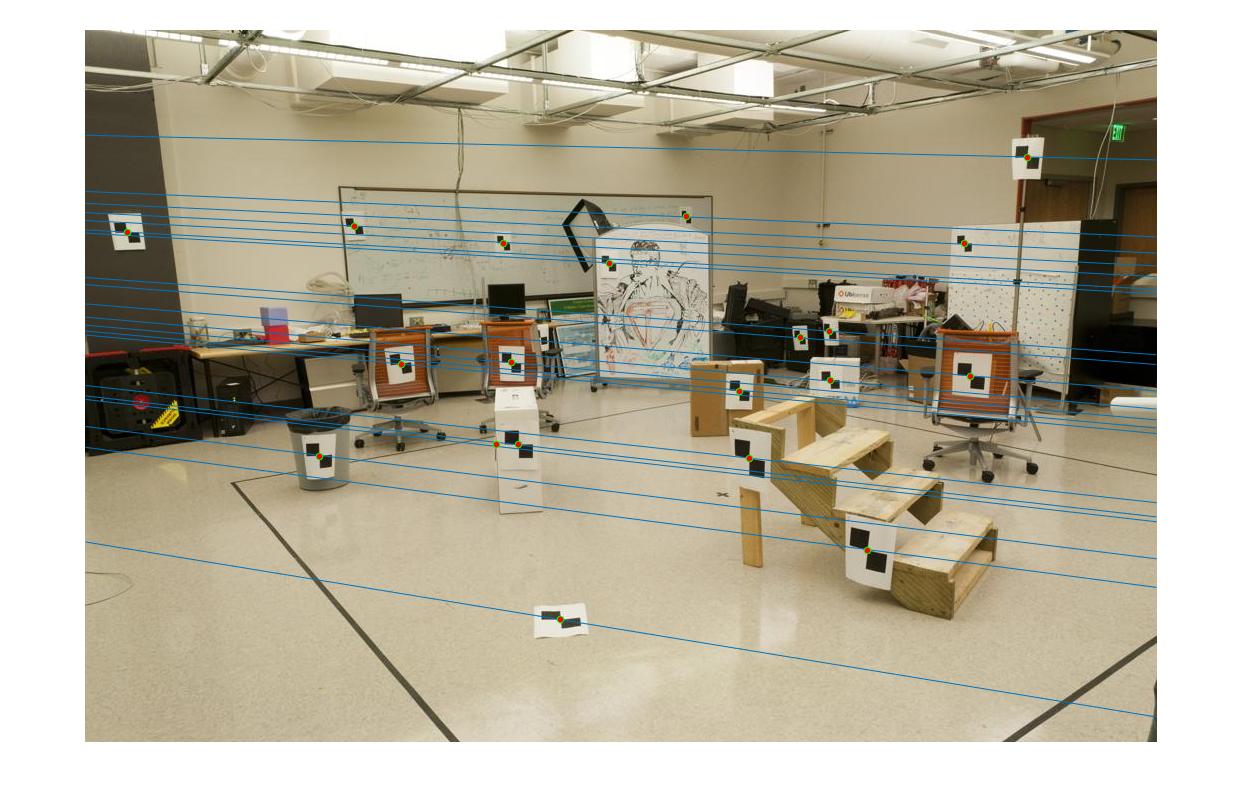
When this part was tested with the two experiment room test images, the resulting epipolar lines calculated from the fundamental matrix did not directly cross through all of the points - which I assume may be due to the large difference and lack of normalization of the points, or because the change to make F rank 2 resulted in some variation and shift in the lines, as the lines did cross through all of the points through the center before rank reduction. However, this problem was fixed by implementing normalization (which was extra credit for this project). The below image shows the results for part 2 (epipolar line estimation for the experiment room/testing image) before normalization.

Point Normalization (Extra Credit)

To improve the estimate of the fundamental matrix, the coordinates in the images can be normalized first - as currently, the points have large and varying magnitudes, with pixel locations as small as single-digit values or as high as the thousands. The normalization process was done by calculating a scale and offset matrix for both of the input images and the their corresponding points that are being used to estimate the fundamental matrix. The two offset matrices contains the mean of the points for image a and image b which is used to determine the offset. The two scale matrices contains a scale multiplier for the points based on the two images, which is calculated by taking one over the standard deviation for each of the respective point groups (a and b). The transformation matrix is the result of the scale matrix dot product with the offset matrix, which results in one for each point group - Transform matrix for A, and Transform matrix for B. After the images are scaled, the fundamental matrix is then calculated, and then finally reverted by simply multiplying the transform matrix for B transposed by the calculated fundamental matrix, and then multiplying that by the transform matrix for A, which results in the fundamental matrix for the original image. The code for this is shown below. By doing this, the accuracy of the fundamental matrix improved greatly on the test image, as the epipolar lines now crossed directly through the given points. This part also helped with the results in the next section greatly, when applied to more real-world image samples. The below image shows the results for part 2 (epipolar line estimation for the experiment room/testing image) after normalization.

Fundamental Matrix with RANSAC

For the final part of this project, the fundamental matrix estimation portion as described in the previous section was put to the test with actual images. First, VLFeat was used to generate features in both images and potential matches between the two images. These point matches were used with RANSAC in order to determine the best fundamental matrix. 8 randomly sampled points were chosen each time per iteration of RANSAC, as 8 point pairs are needed to estimate the fundamental matrix. The number of iterations to do for RANSAC varied per image for the results shown here, but in general, we wanted the probability of choosing 8 points that were non-outliers to be 99%, and we assumed that roughly 60% of our image point correspondences returned by VLFeat were outliers (meaning that they are incorrect). For each iteration, these 8 points were used to calculate the fundamental matrix. To determine how accurate this fundamental matrix truly is, we counted how many inliers out of all the matches returned by VLFeat resulted from using the currently calculated fundamental matrix. To determine if a match was an inlier, we used the main property of the fundamental matrix (x_b' * F * x_a = 0) and determined a distance property to 0 for each image pair. For example, if the threshold was 0.003, this means that if a match resulted in x_b' * F * x_a <= 0.003, the match was classified as an inlier. After all iterations of RANSAC had completed, the fundamental matrix that resulted in the highest number of inliers was chosen as the final fundamental matrix. The top thirty to fifty matches (with the lowest distance score) were then displayed to the user. A 0.003 threshold was generally used as a default, but based on the number of inliers returned, the number was then callibrated.

However, for a lot of real images, the resulting fundamental matrix that was estimated may be wrong. However, even if the resulting fundamental matrix is wrong, they still manage to remove many incorrect matches, but will likely also take many correct matches out with them. Below is the code for RANSAC.

Results for Part 3

A large variety of examples are shown below. All images are done with normalization of points unless otherwise specified. The top fifty matches for each image are shown below.

Mount Rushmore

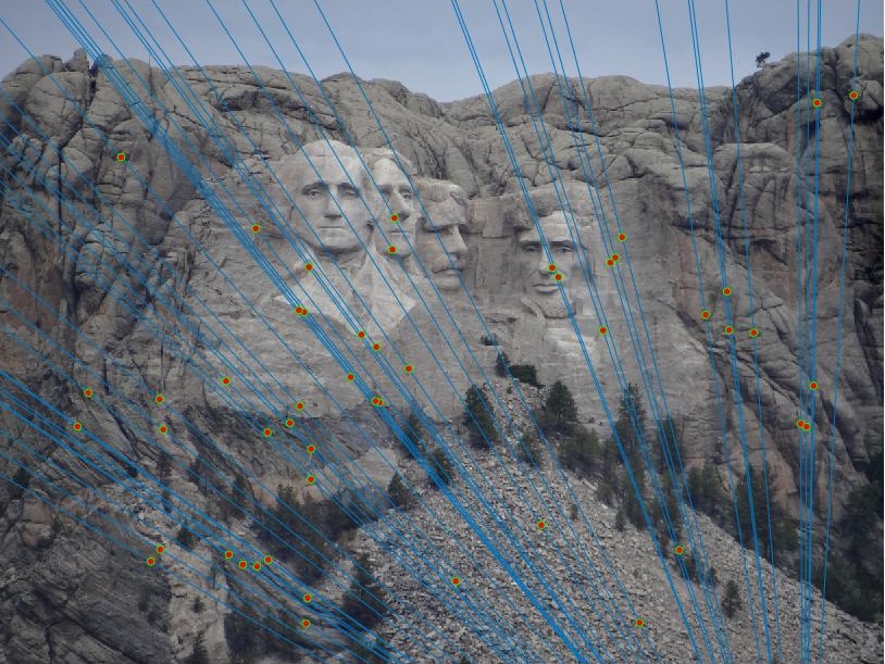
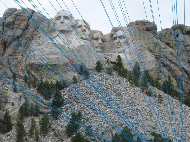
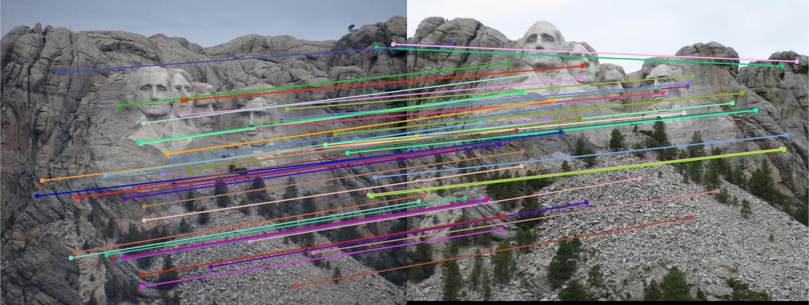
Of the top 50 matches, it appears that most of the matches seem to be accurate. VLFeat's original matches for Mount Rushmore were also very accurate, as with a threshold of 0.005 most were deemed as inliers (roughly 600 out of the 1000 were deemed as inliers with the current threshold). Even with a relatively high threshold for this image, the matches generated seem to be very accurate when ordered by lowest distance.

Notre Dame

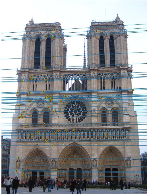
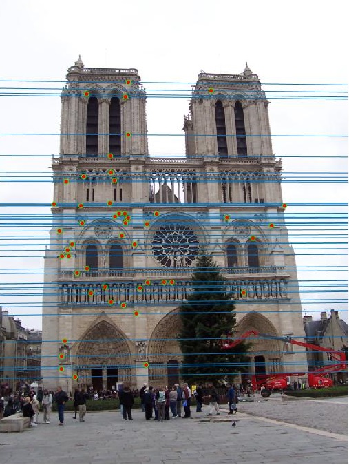
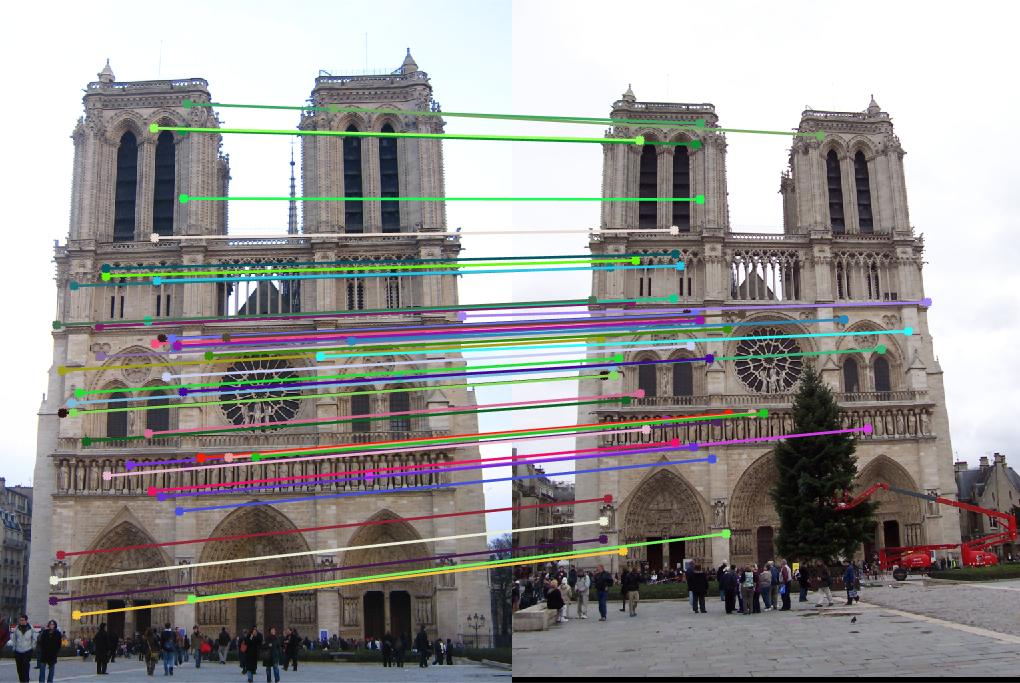
Of the top 50 matches, most of these matches also seem to be accurate. VLFeat's original matches also seemed to be fairly accurate for this pair.

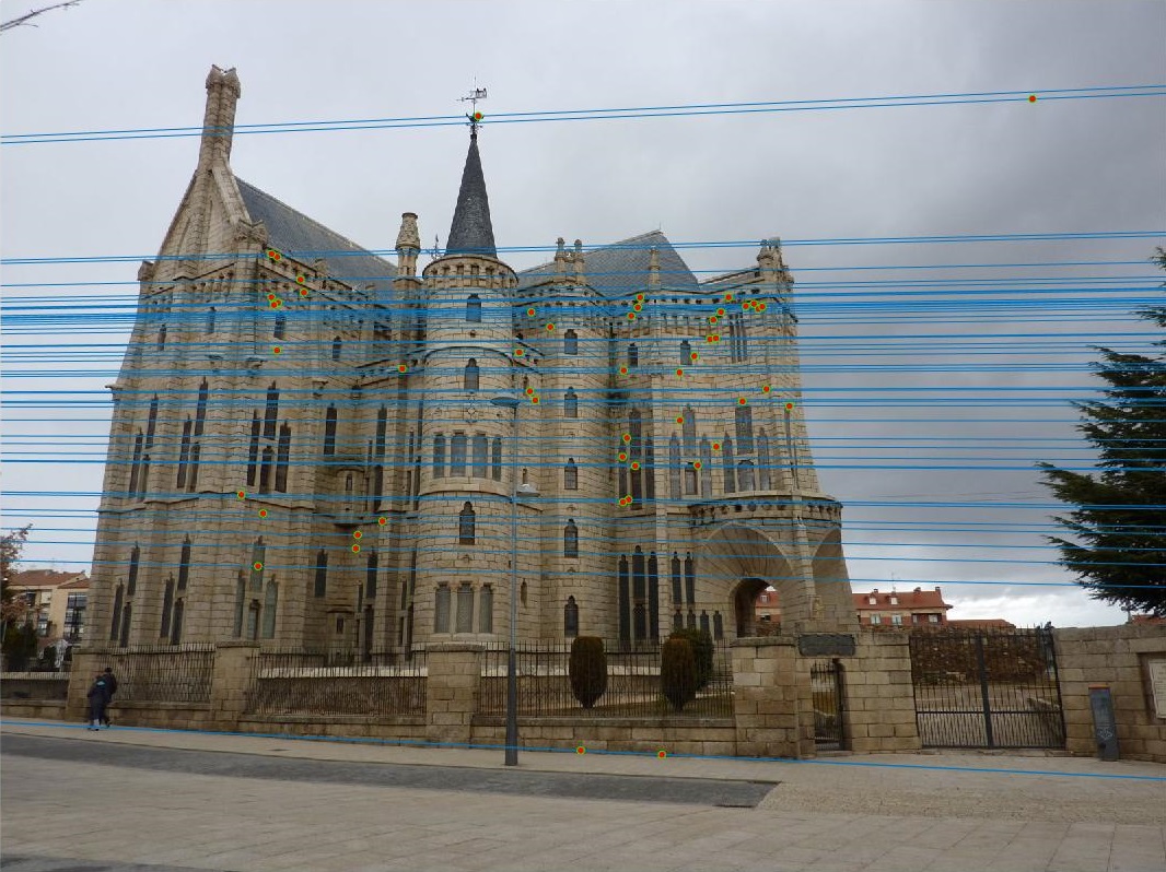
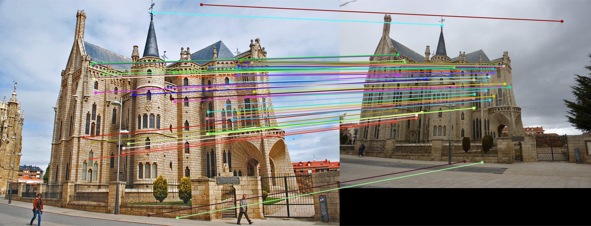
Episcopal Gaudi - Without Normalization

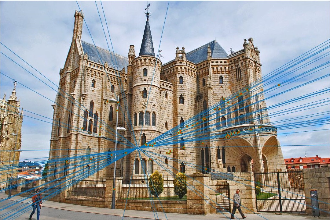
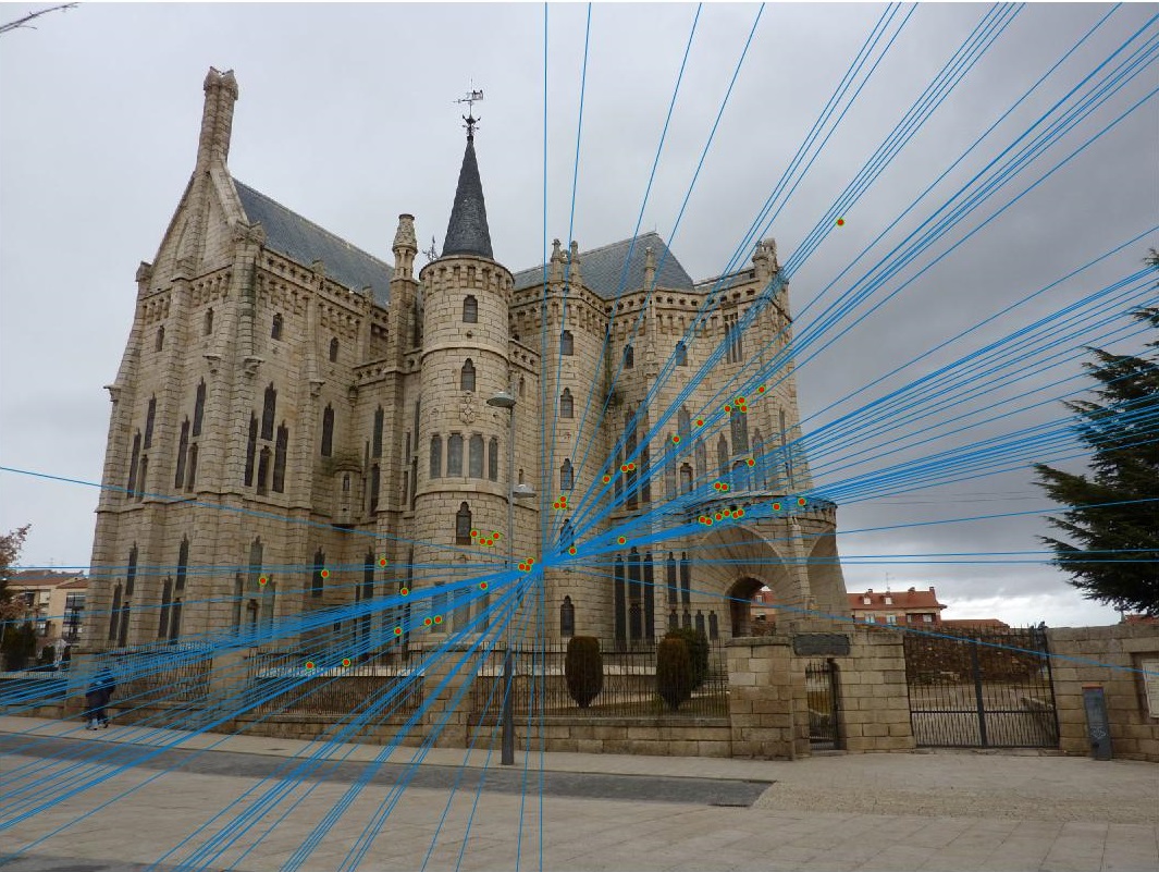
Episcopal Gaudi without normalization in the calculation of the fundamental matrix proved to be quite messy, with a noticeably large amount of points still being outliers. This filtering is definitely more accurate than what was done in the last project without scene geometry, but could still use improvement.

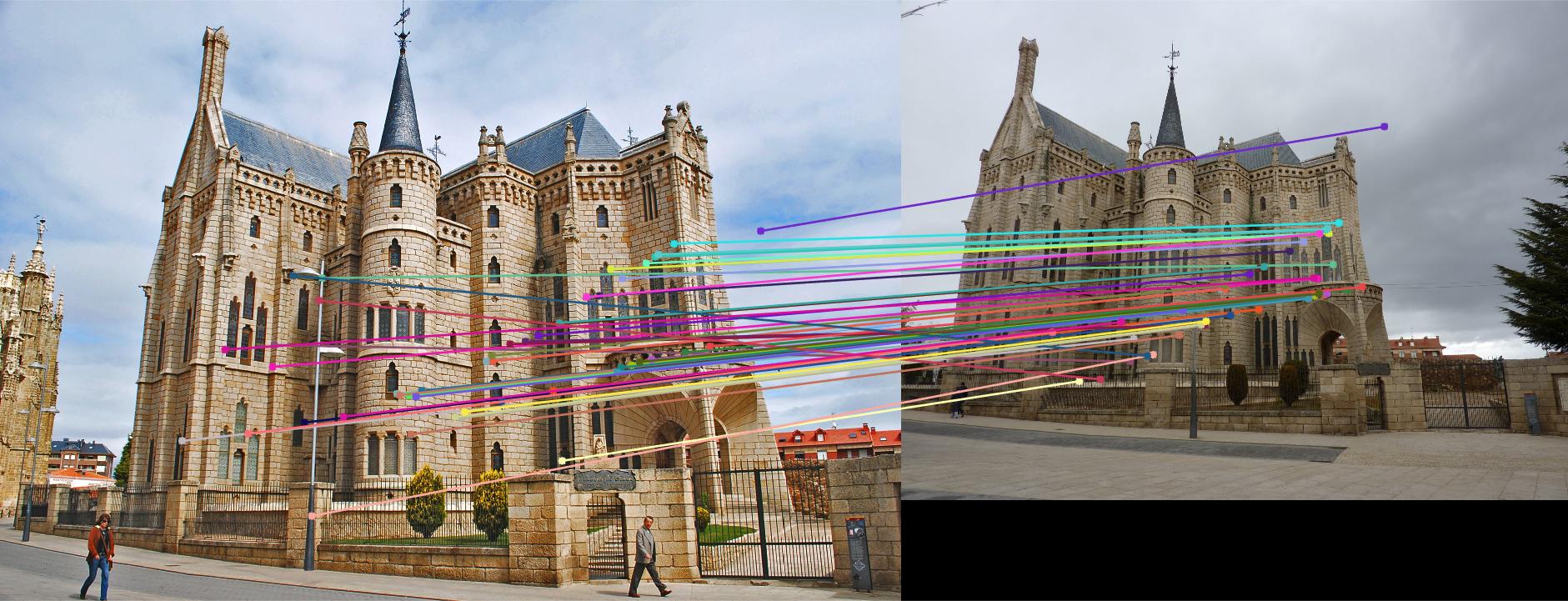
Episcopal Gaudi - With Normalization

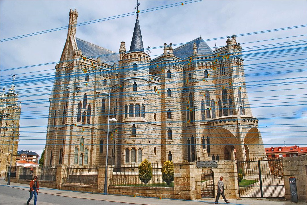
Episcopal Gaudi with normalization in the calculation of the fundamental matrix proved to be show a much larger improvement with a threshold of 0.003. Most of the images (if not all) appear to be inliers this time, showing how the normalization process can help improve the accuracy of the fundamental matrix by a lot.

Woodruff

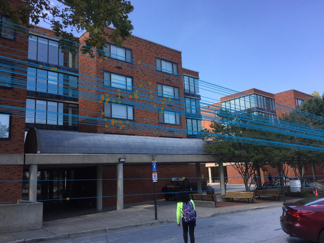
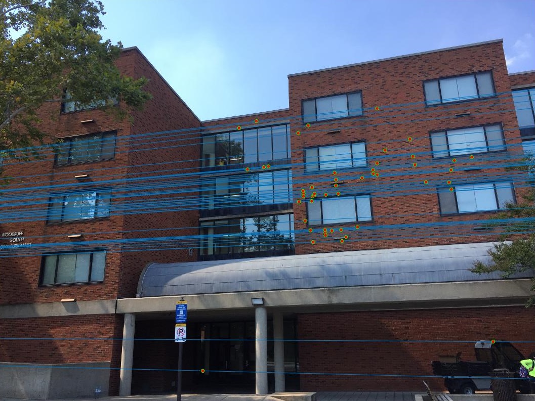
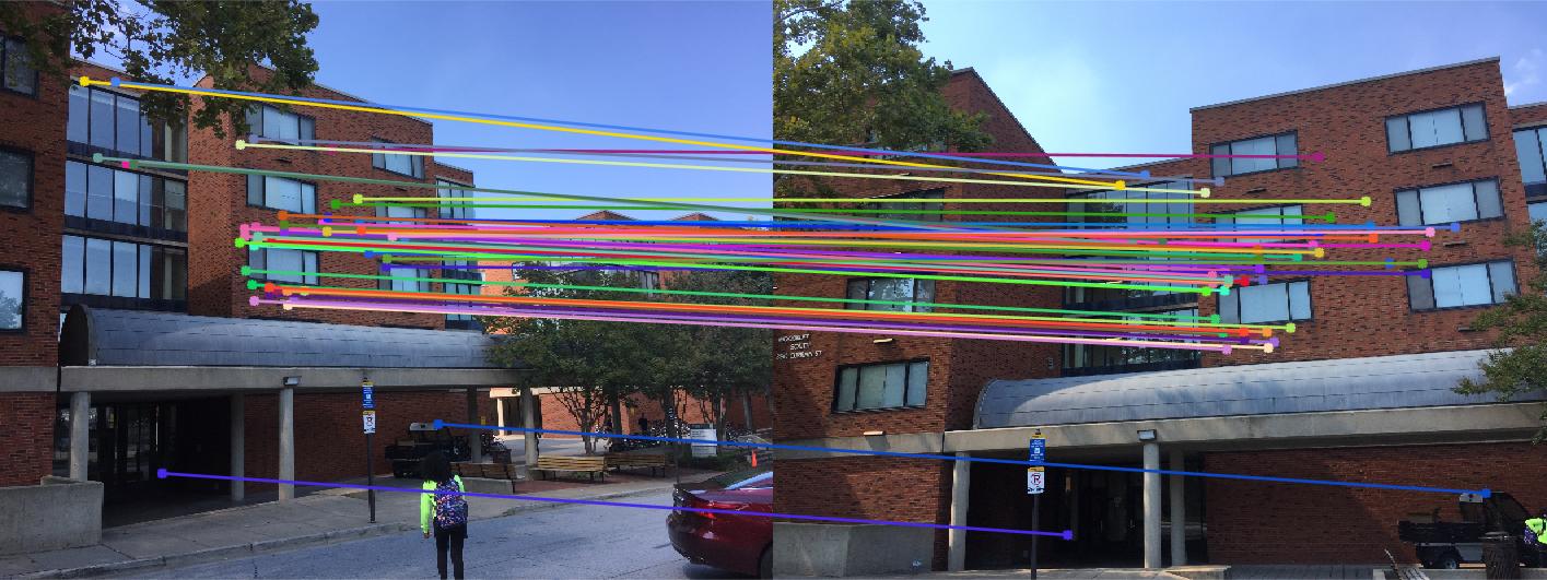
Woodruff shows pretty accurate matches overall, with the epipolar lines also corresponding to the geometry of the scene pretty well (notice how they go in alignment with the building).

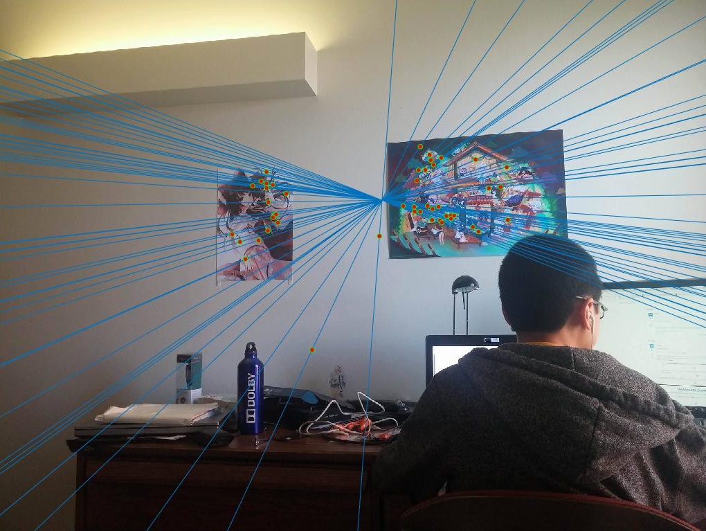
Roommates 1

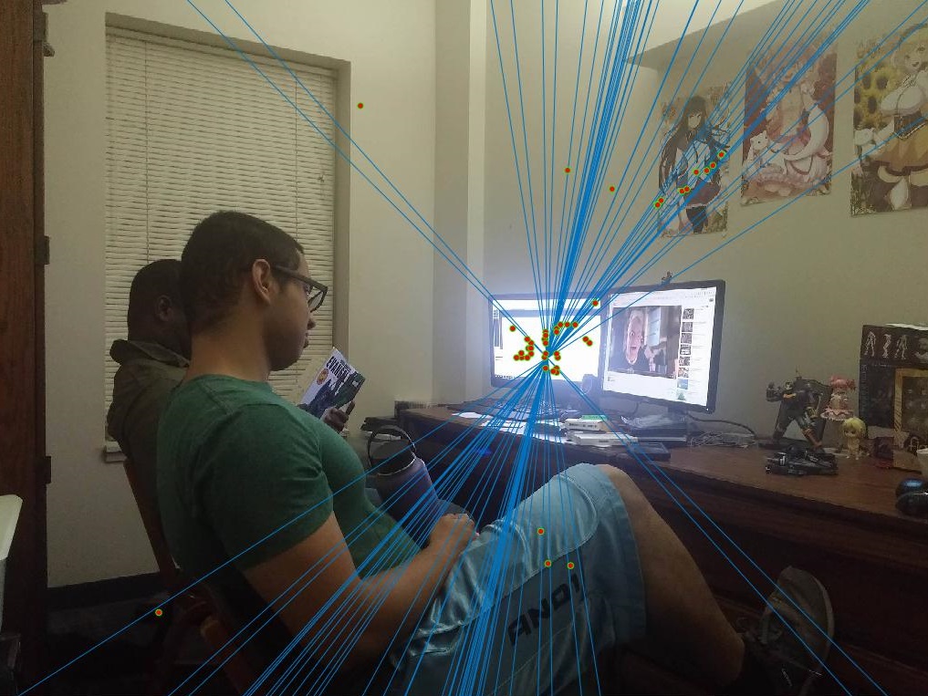
This pair of roommates did not do as well as the previous examples, with some points blatantly wrong and some others, even though grouped in the right general direction, still somewhat off. Most of the points seemed to be clustered around the monitor, even though it appeared to be mostly one color - maybe there's distinct noise over there? The poster matches do seem pretty accurate, however.

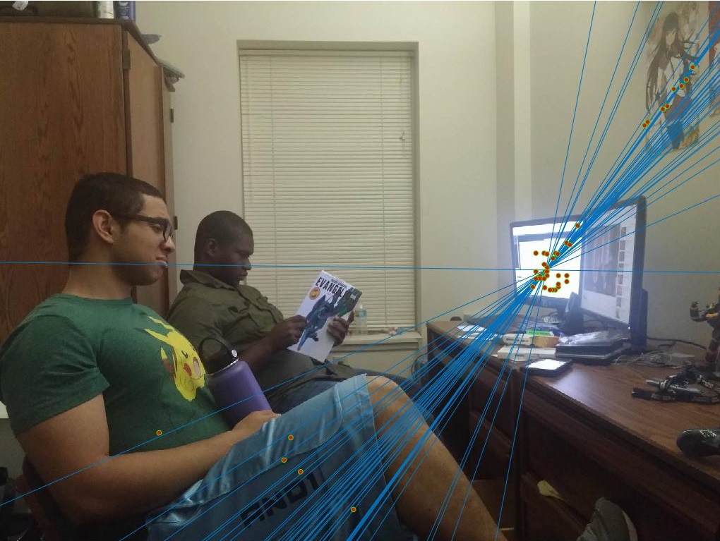
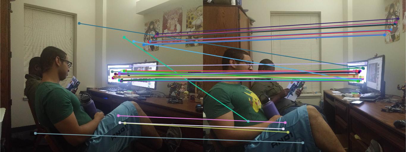
Roommates 2

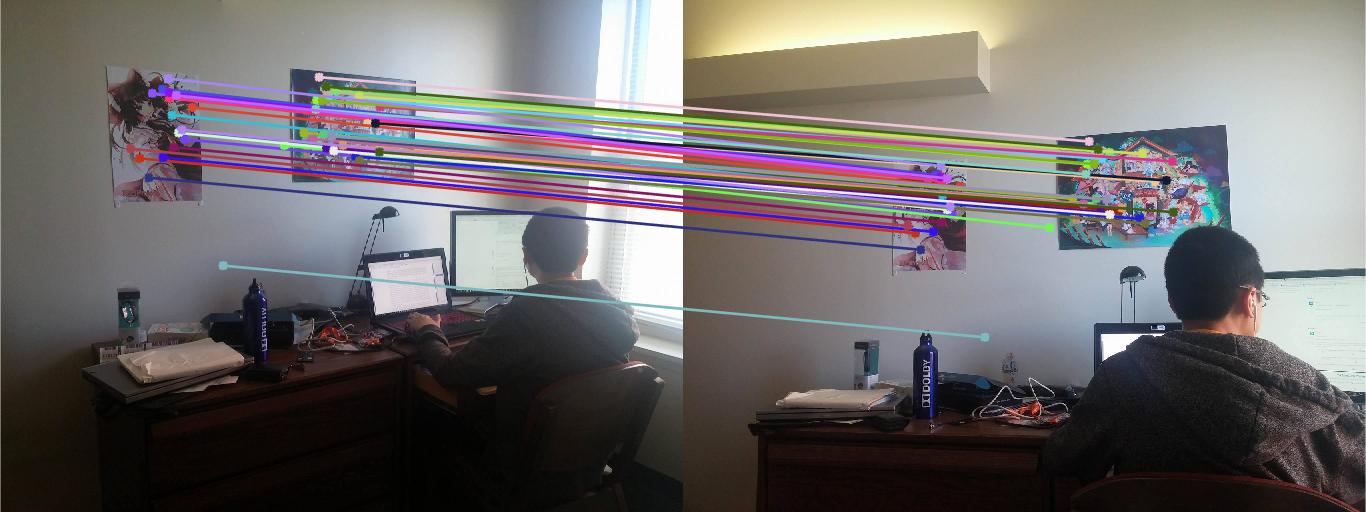
This one did pretty well overall, but it once again matched most of the points from the poster. Most points seem to be matched up correctly.

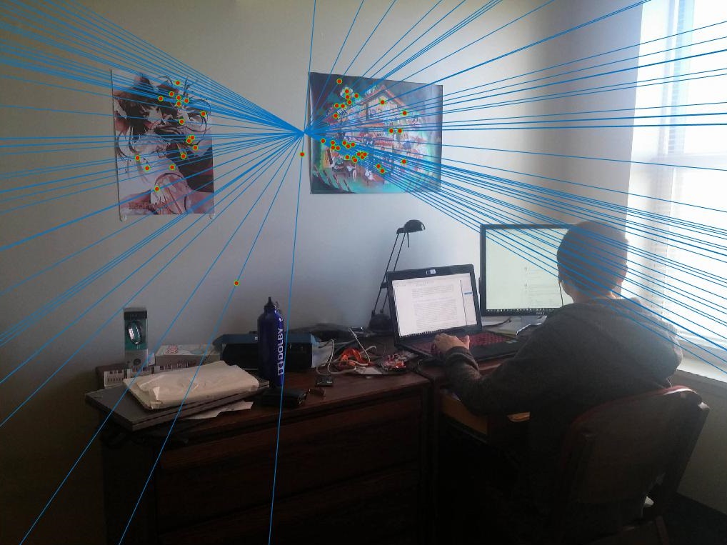
Posters

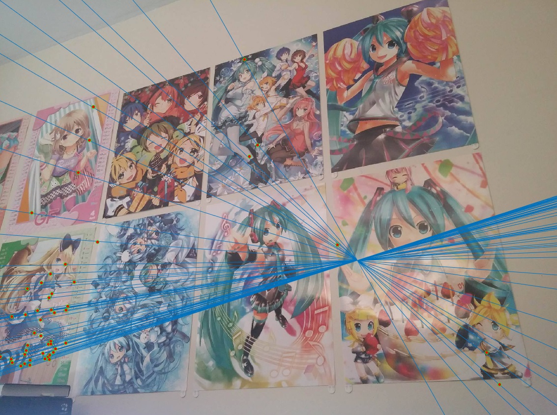
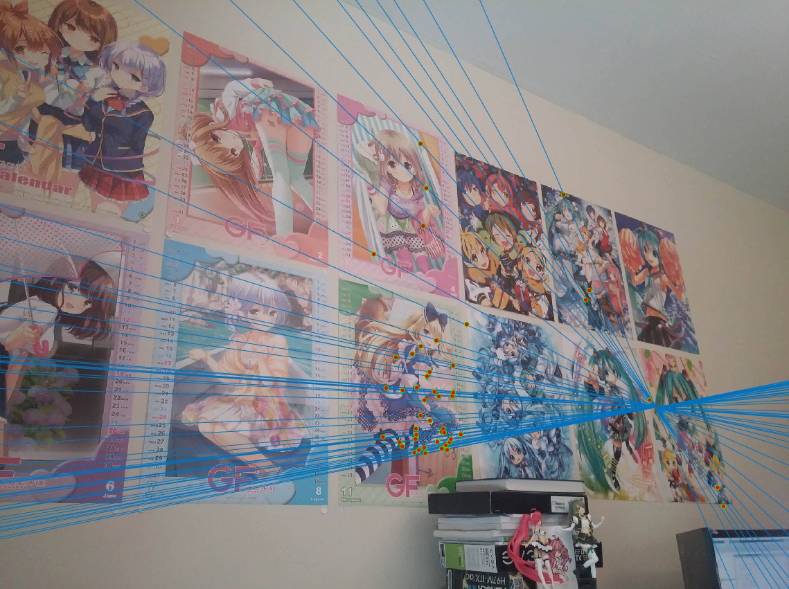
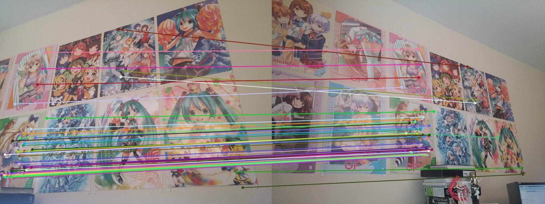
This one did pretty well overall, although the epipolar lines are not what I what have expected - something more similar to Woodruff was expected. But since most were non-man made images, it may have been difficult for it to recognize.

Cherry Blossoms

This one also did pretty well for the most part, but the original image matching from VLFeat also seemed pretty accurate to begin with.

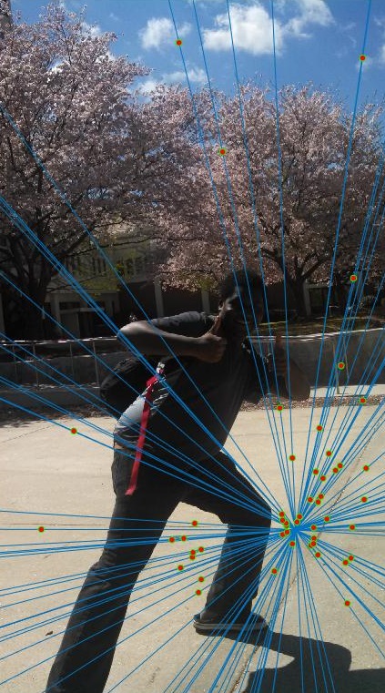
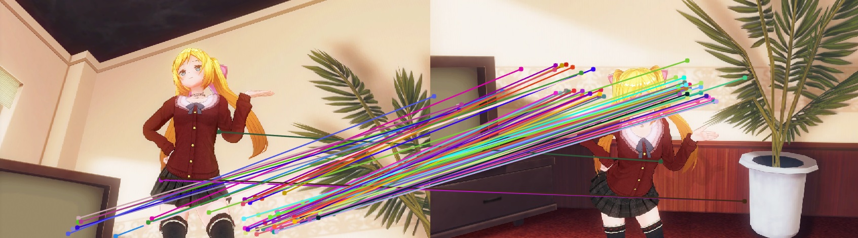
3DCG 1

The 3DCG worked well too, barring one blatantly obvious error. Most of the points detected were from the poles (structural beams), and it did manage to match up most of them correctly.

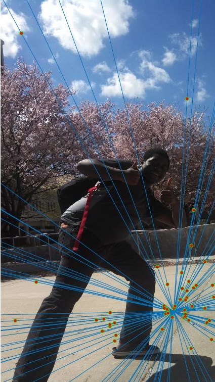
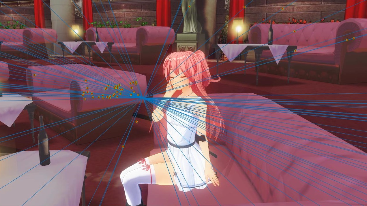
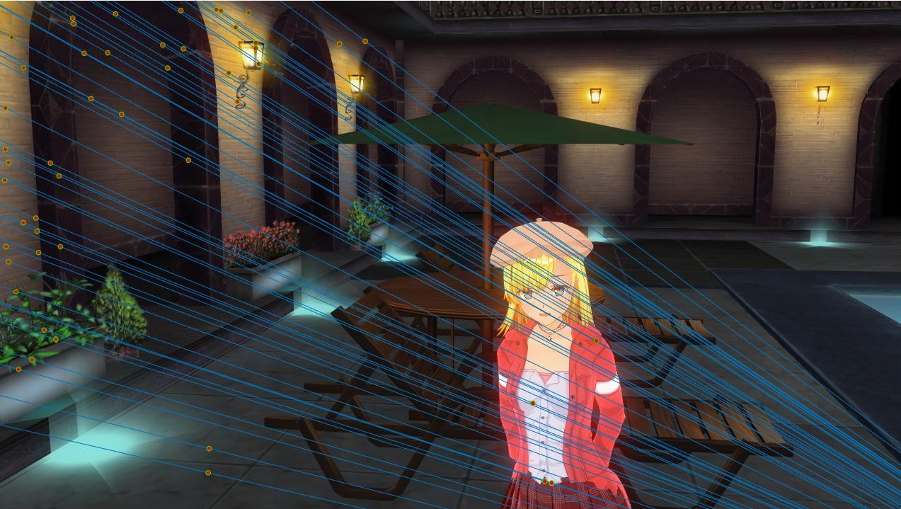
3DCG 2 - Without Normalization

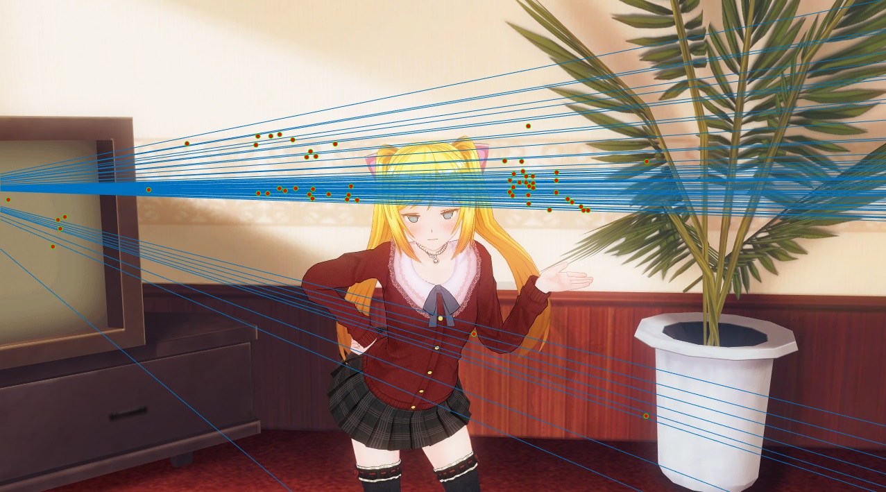
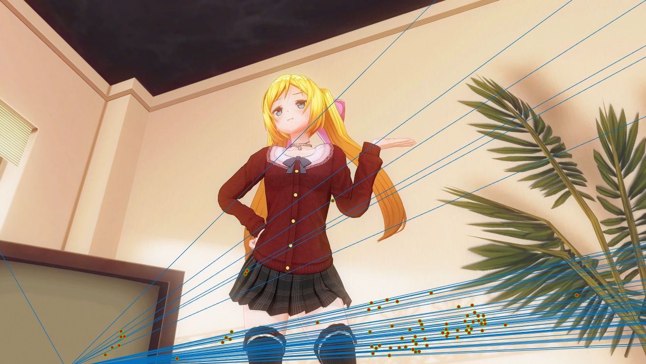
This image pair did not work at all in the last project, but now seems to work somewhat better. Most of the points comes from the strip of patterned design on the wall. After normalization of the fundamental matrix, however, this image pair did a lot poorly even after many tries and a higher number of RANSAC iterations. This may be due to the fact that these images are not from the real world, as the other image pairs have shown improvements.

3DCG 3

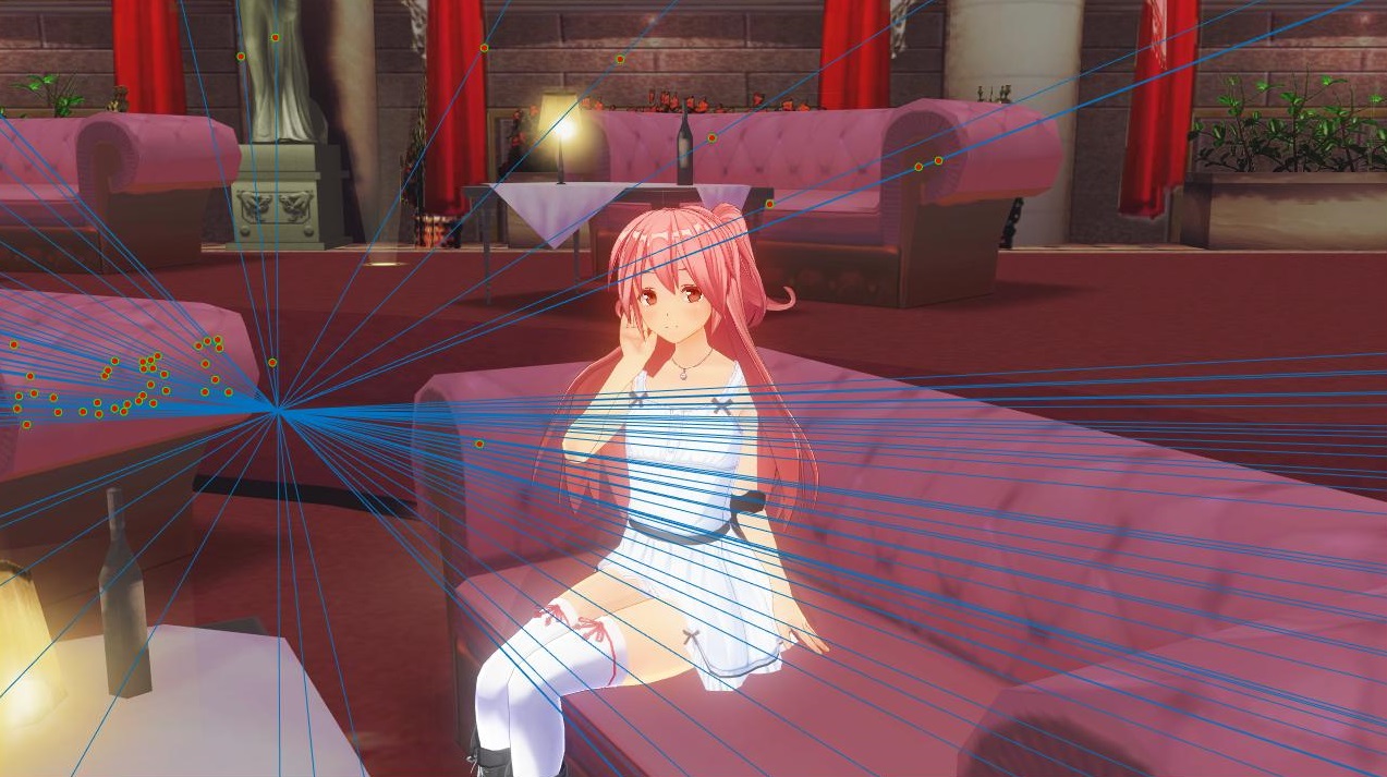
This image pair did fairly well, with some outliers pointing to the wrong couch. Most of the points were clustered from one couch arm, but a few points were also shown from the back that also matched up well. It seems like this algorithm, for non real images, tends to cluster on small yet intricate patterns that are not as noticeable to the human eye for feature matching.

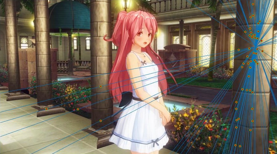
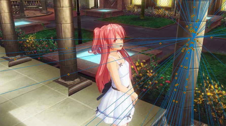
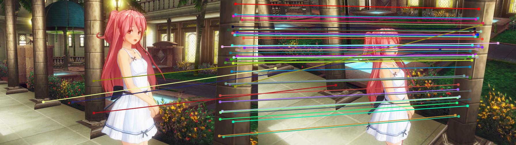
3DCG 4

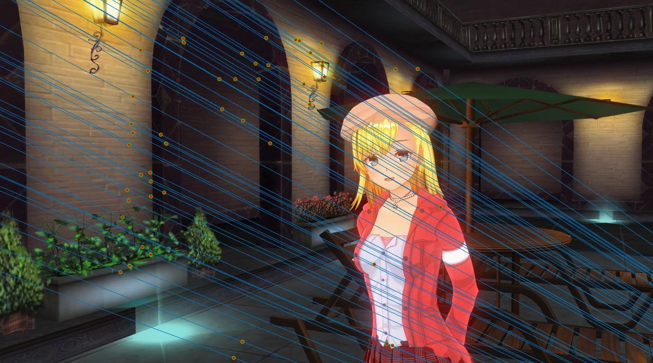
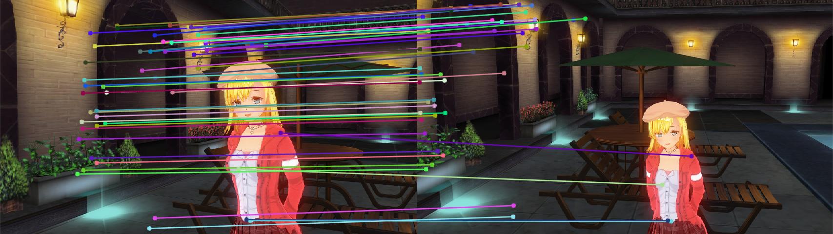
This image pair did very well, with most of the points coming from the arches in the background.