Jonathan Hunter

Fundamental Matrix

Camera Calibration

I solved for the projection matrix by simply using Matlab's least squares regression solver to solve Ax=y. Where A was made using equations provided on the assignment description and y was the set of 2d points. I then solved for the camera center by doing -Q^-1 * m4 as shown on the class slides.

Camera calibration code

% finding the projection matrix M
M = A\Y;
M = [M;1];
M = reshape(M,[],3)';

% finding camera center
Q = M(1:3,1:3);
negQ = -Q;
invQ = inv(negQ);
m4 = M(1:3, 4);
Center = invQ * m4;

Results in a table

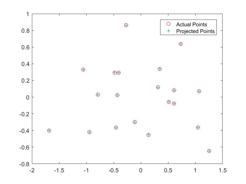
Shown above are the results for running the algorithm on the two provided images. Image 1 had the following results:

The projection matrix is:
    0.7679   -0.4938   -0.0234    0.0067
   -0.0852   -0.0915   -0.9065   -0.0878
    0.1827    0.2988   -0.0742    1.0000


The total residual is: <0.0445>

The estimated location of camera is: <-1.5126, -2.3517, 0.2827>

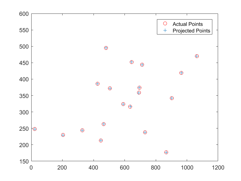
Image 2 had these results:

The projection matrix is:
   -2.0466    1.1874    0.3889  243.7330
   -0.4569   -0.3020    2.1472  165.9325
   -0.0022   -0.0011    0.0006    1.0000


The total residual is: <15.6217>

The estimated location of camera is: <303.0967, 307.1842, 30.4223>

Image 1 had results that were exactly as expected and even though Image 2 had a high residual it matched to the points fairly well.

Fundamental Matrix

I solved for the fundamental matrix using Matlab's SVD solver to solve for Af = 0 where A was created using the equations on the slides from class. I then used SVD again to convert the solved fundamental matrix to a rank 2 matrix.

Fundamental matrix code

% solve Af = 0
[U, S, V] = svd(A);
f = V(:, end);
F_matrix = reshape(f, [3 3]);

% reduce the rank of F
[U, S, V] = svd(F_matrix);
S(3,3) = 0;
F_matrix = U*S*V';

I also solved for the normalization of F by finding the mean values for u and v in both sets for the translation component. I then used those mean values to solve for the mean squared distance and set the scaling to make that value equal to 2.

Normalization code

% find Ta
a_c_u = mean(Points_a(:,1));
a_c_v = mean(Points_a(:,2));
s_a = 2 / sqrt(a_c_u^2 + a_c_v^2);
Ta = [s_a 0 0; 0 s_a 0; 0 0 1] * [1 0 -a_c_u; 0 1 -a_c_v; 0 0 1];

...

% Undo the normalization on F
F_matrix = Tb' * F_matrix * Ta;

Results in a table

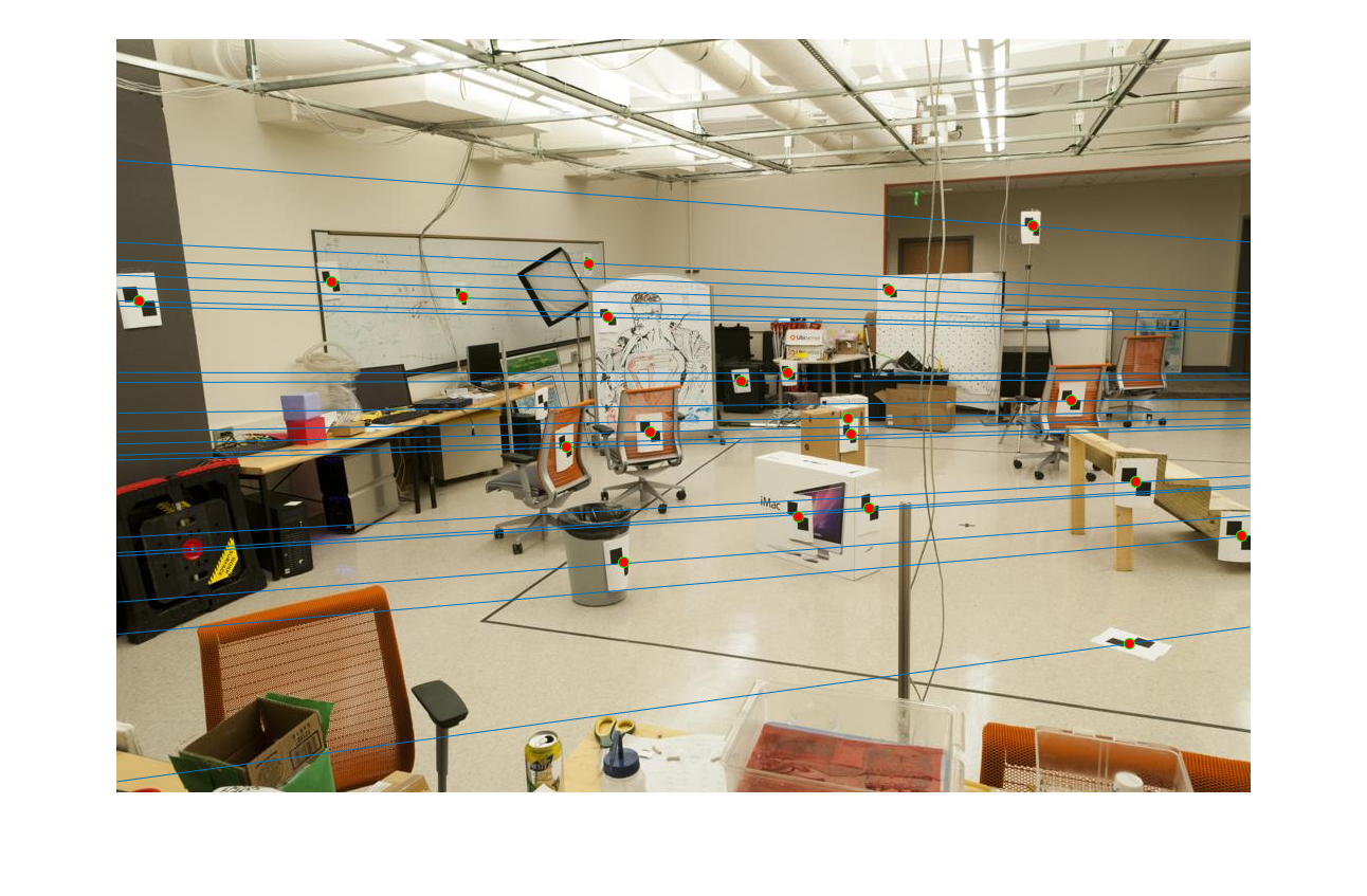
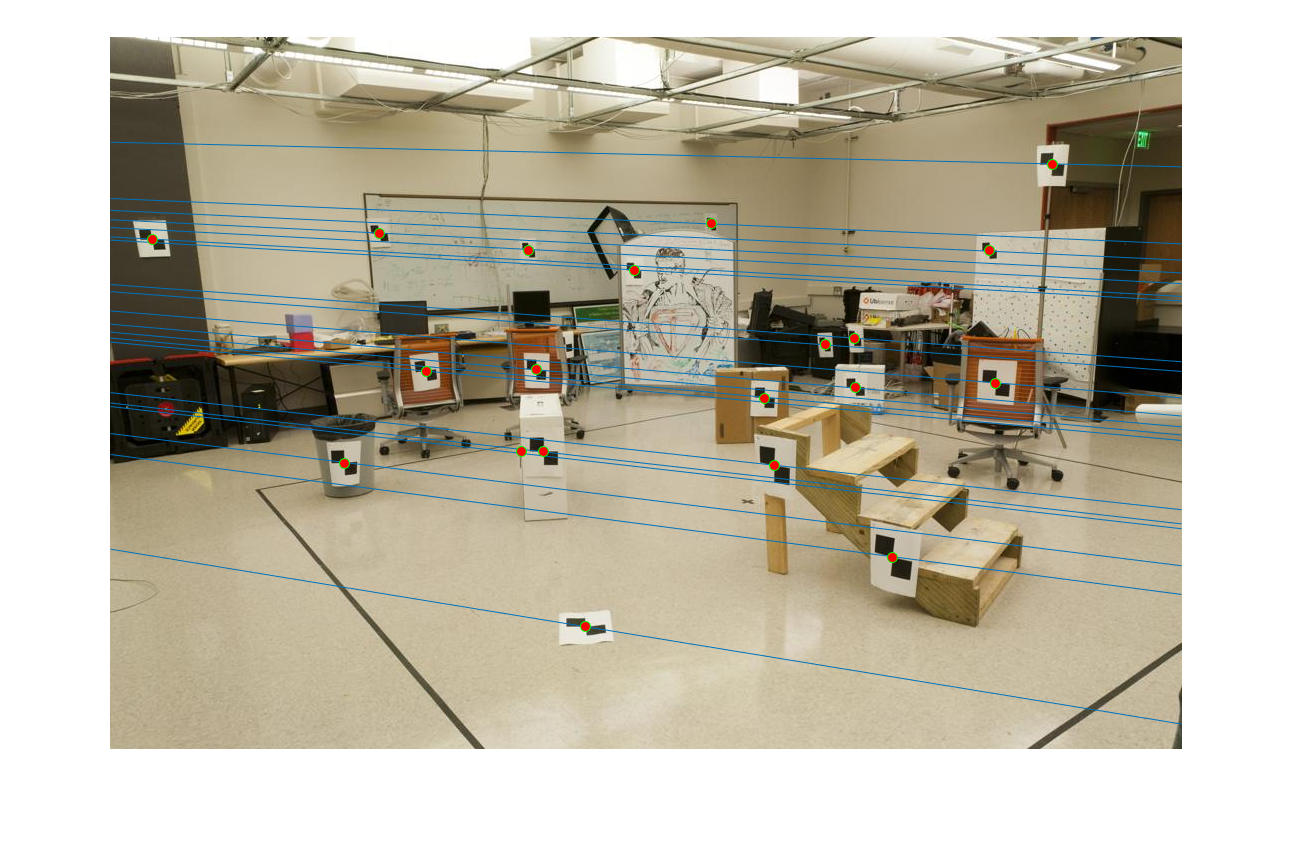
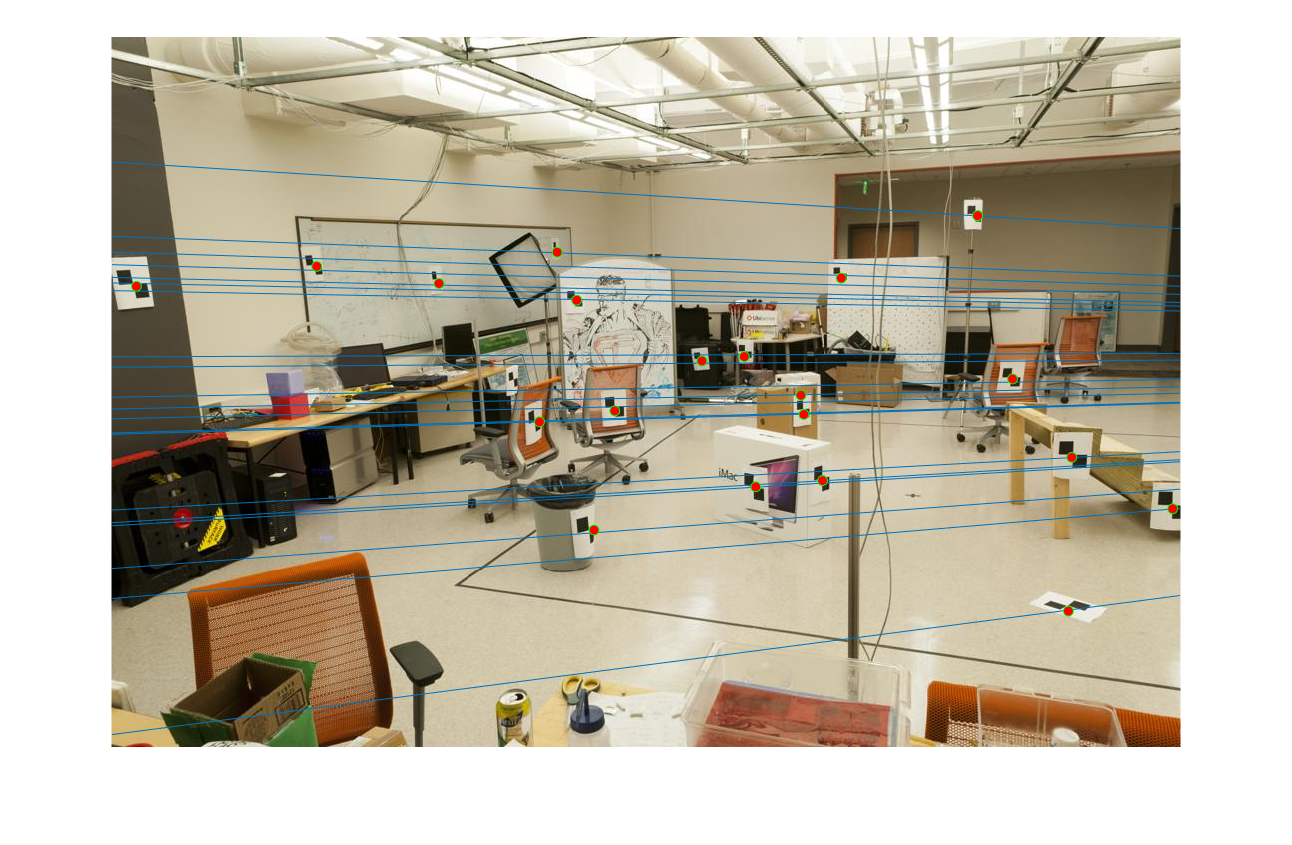
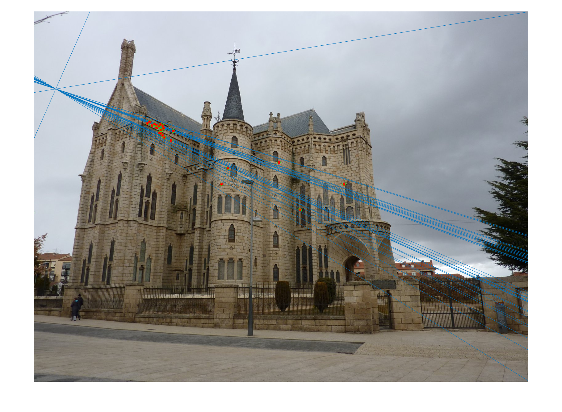
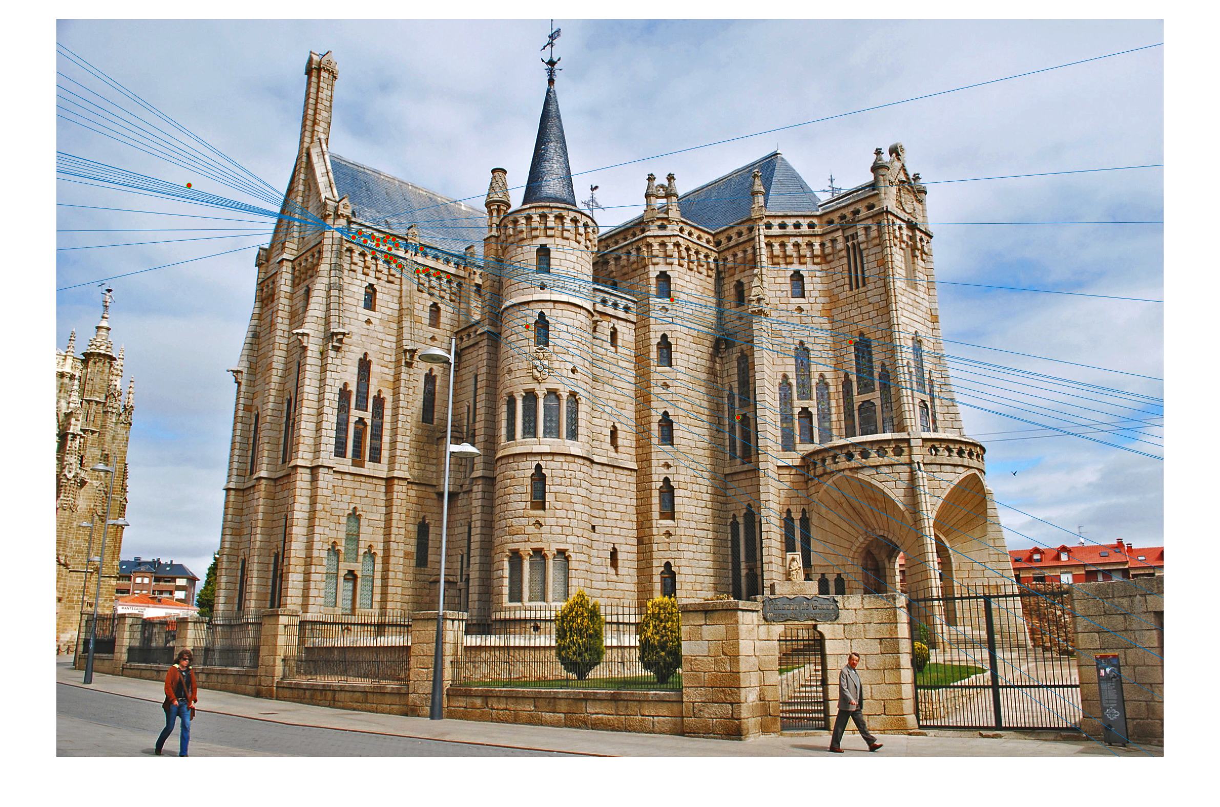
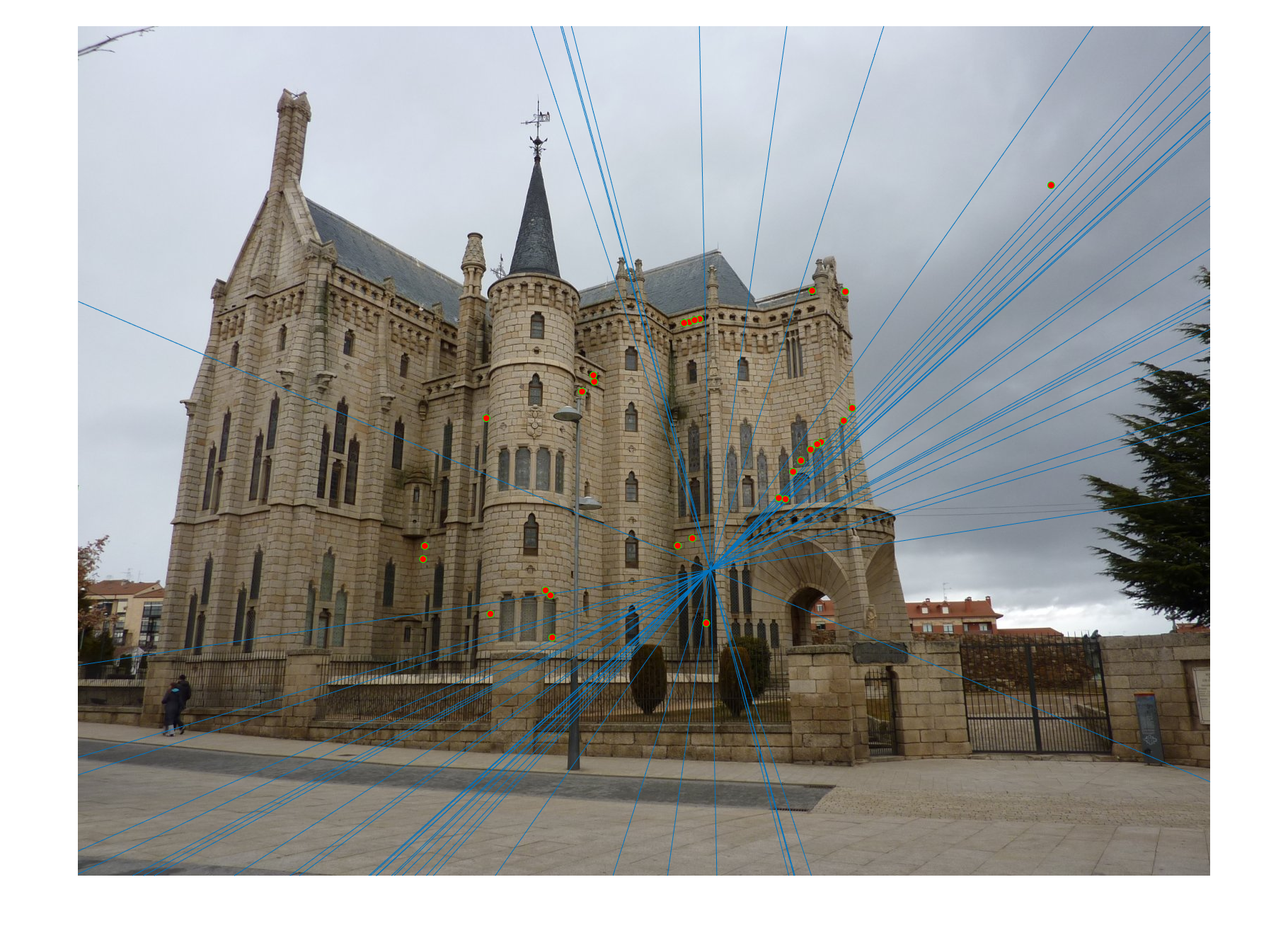
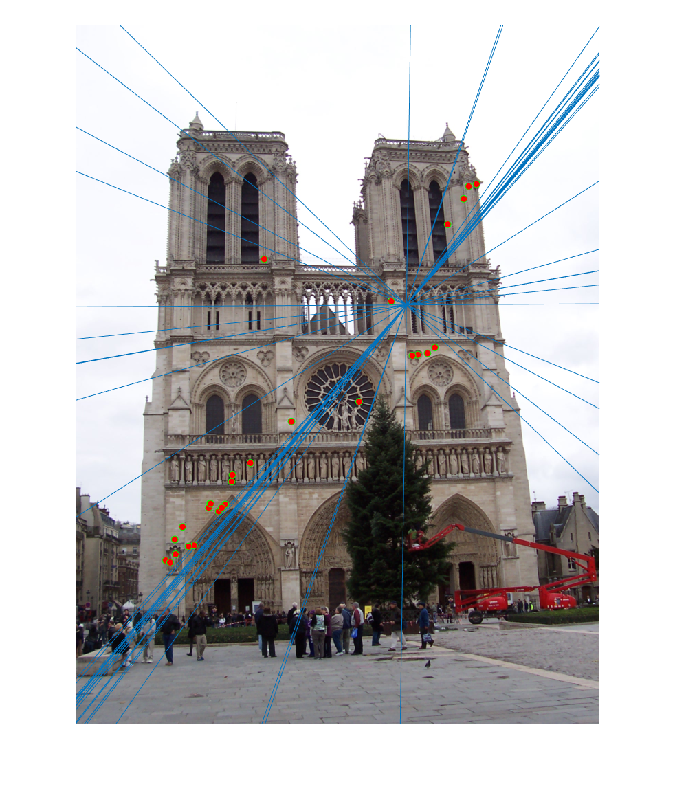
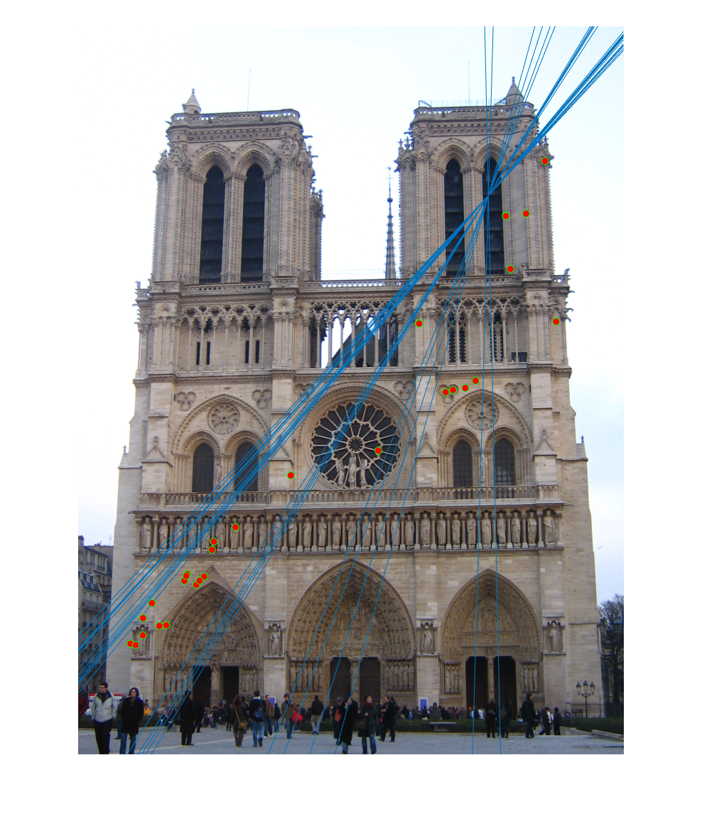
The first row shows running the code with normalization and the second without. As can be seen in the images, the epipolar lines match up much more closely with the normalization than without.

RANSAC

I implemented RANSAC using the following code:

RANSAC code

for i = 1 : 2000
   % Sample
   samples = randsample(dim(1), 8);
   samples_a = matches_a(samples, :);
   samples_b = matches_b(samples, :);
   
   % Solve
   current_f = estimate_fundamental_matrix(samples_a, samples_b);
   
   % Score
   current_inliers = 0;
   current_inliers_a = zeros(dim);
   current_inliers_b = zeros(dim);
   current_confidences = zeros(dim(1));
   for j = 1 : dim(1)
      a = matches_a(j, :);
      b = matches_b(j, :);
      a = [a(:);1];
      b = [b(:);1];
      error = abs(a' * current_f * b);
      if error < .01
         current_inliers = current_inliers + 1; 
         current_inliers_a(current_inliers, :) = matches_a(j, :);
         current_inliers_b(current_inliers, :) = matches_b(j, :);
         current_confidences(current_inliers) = error;
      end
   end
   if current_inliers > best_inliers
       Best_Fmatrix = current_f;
       best_inliers = current_inliers;
       inliers_a = current_inliers_a;
       inliers_b = current_inliers_b;
       confidences = current_confidences;
   end
end

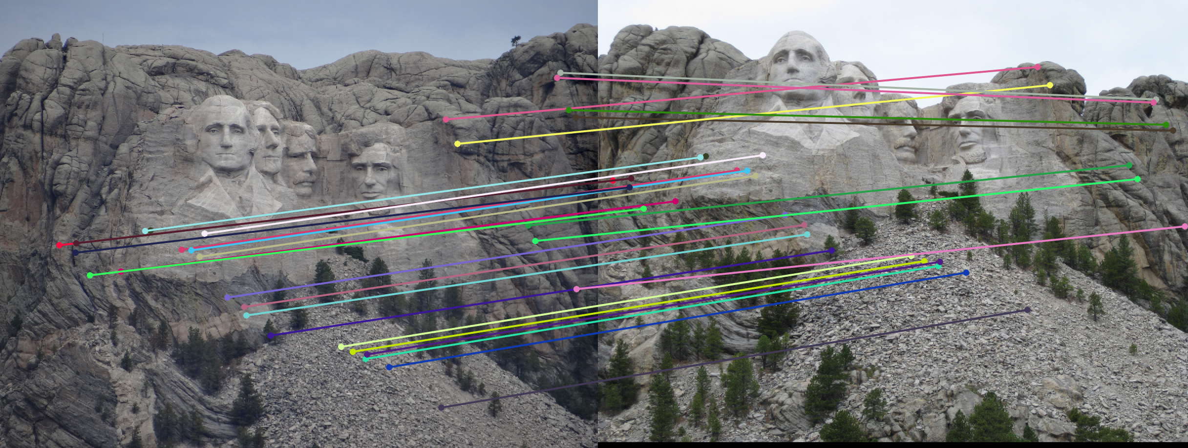
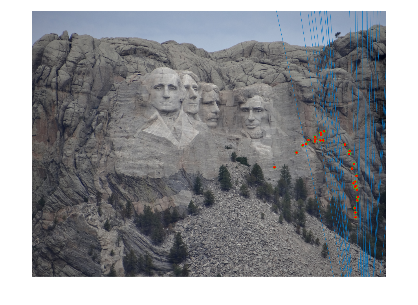
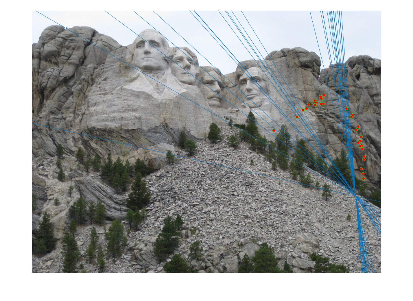
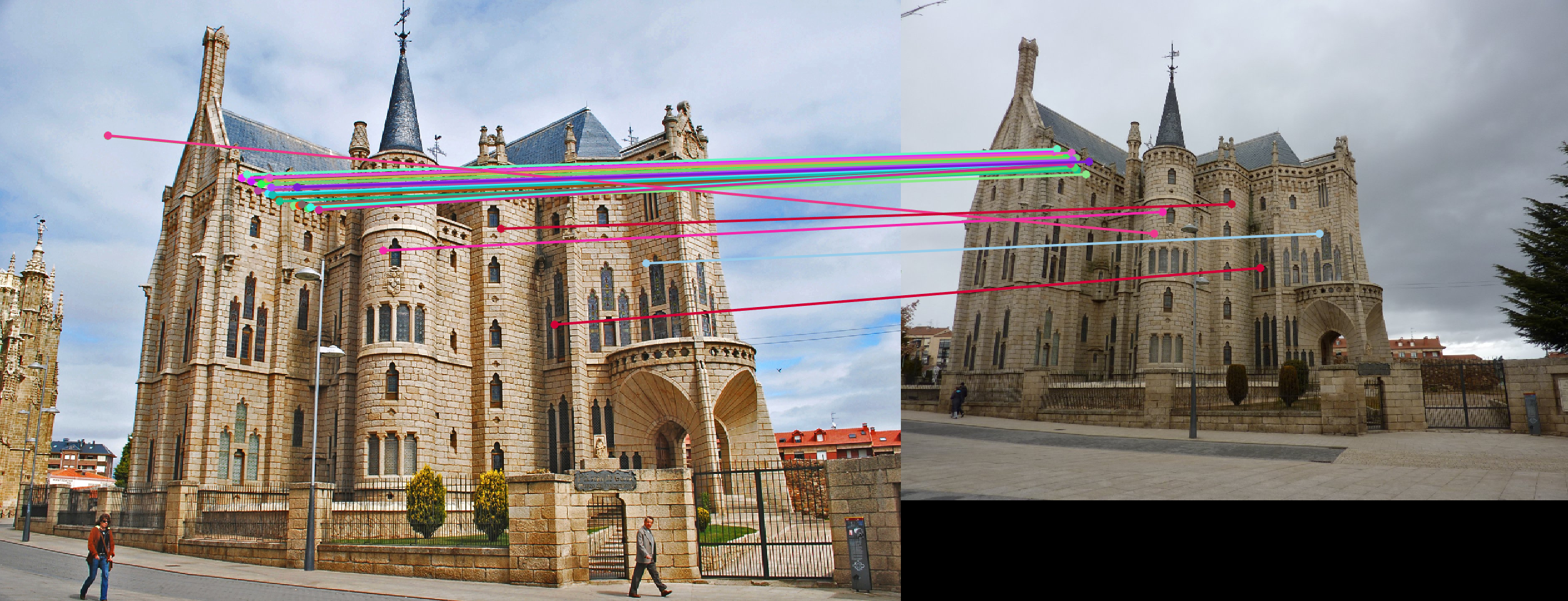
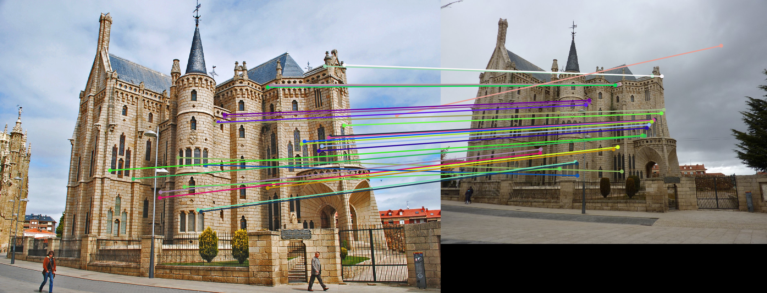
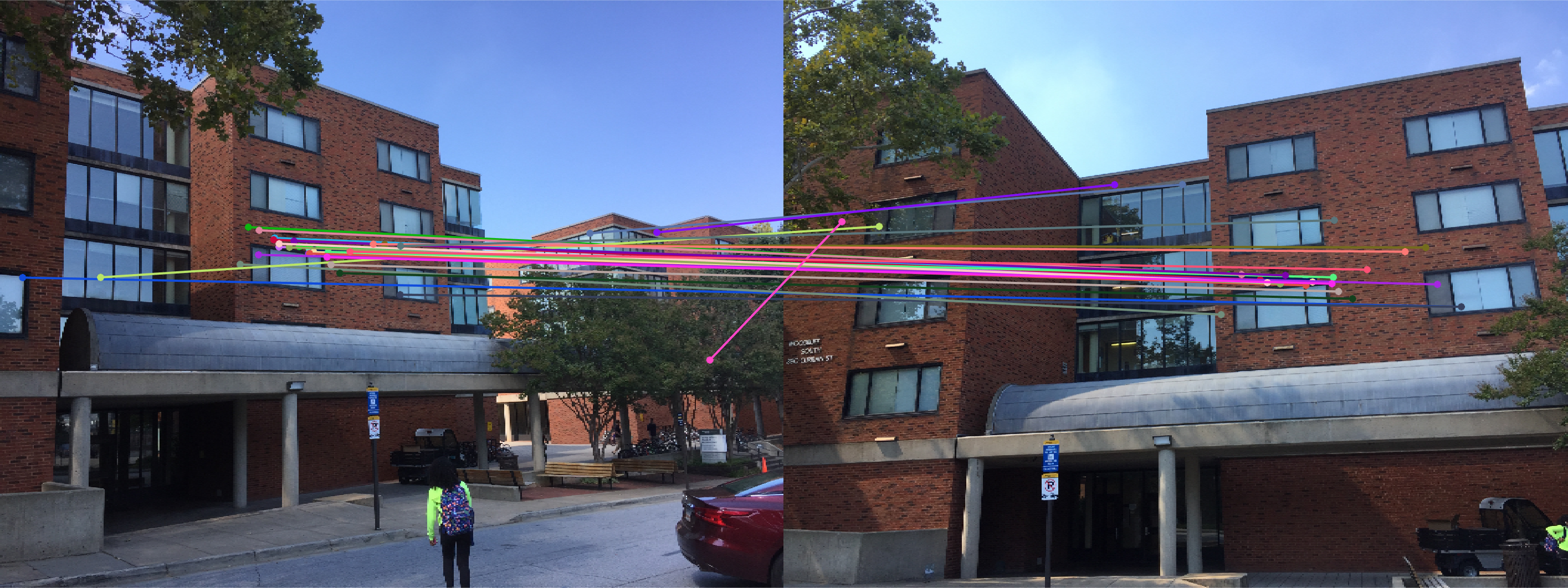
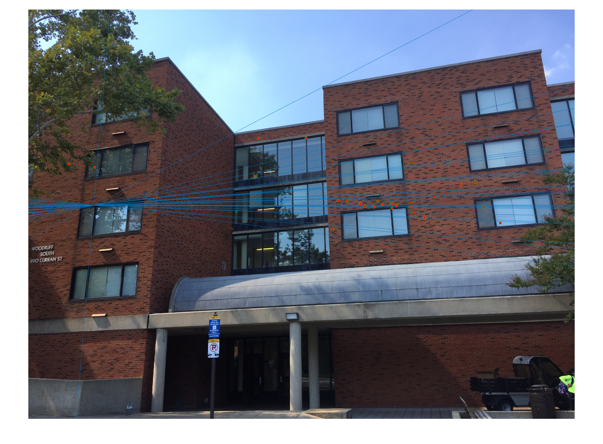
I first use randsample() to get 8 numbers to use as samples for finding a fundamental matrix. Then I find inliers using the x^T * F * x' = 0 property of the fundamental matrix. Since that value should be 0 I used how close that was to 0 as my confindence metric. I chose a cutoff of .01 as that seemed to produce ~150 inliers per run of the algorithm. The rest of the score section just saves the matrix with the highest amounts of inliers. However, before returning inliers_a and inliers_b I sort them based on the confidences I calculated and only return the top 30.

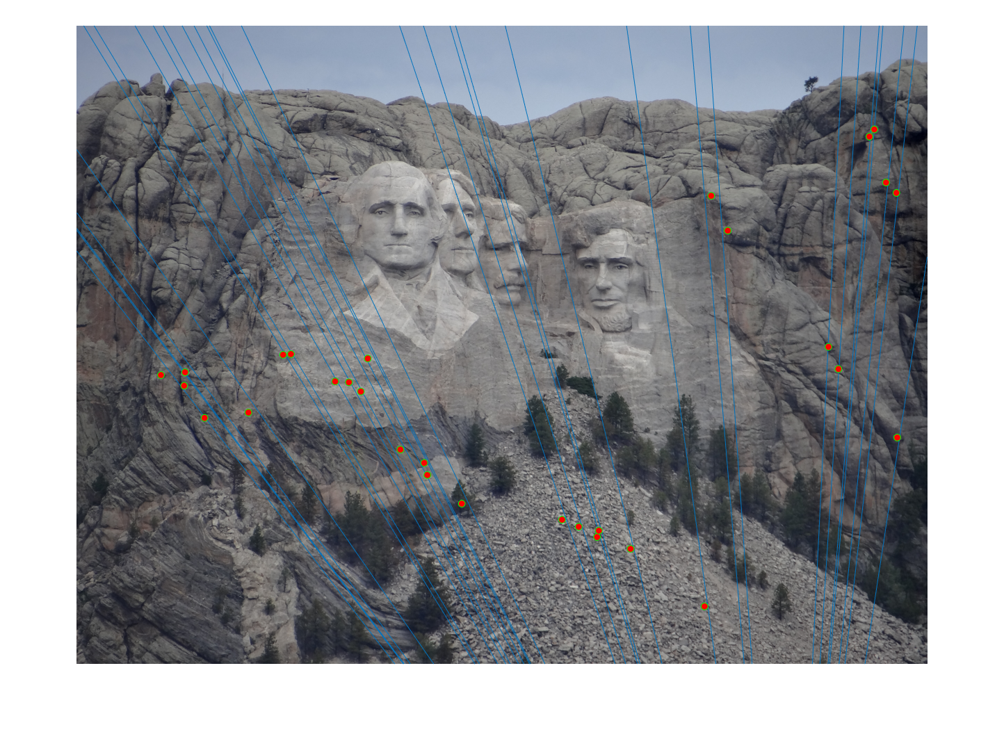
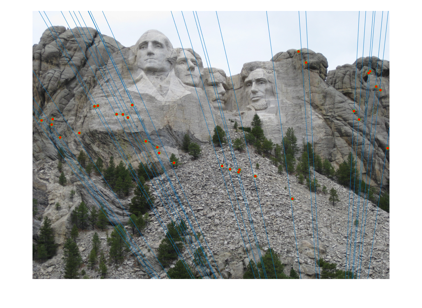
Results in a table

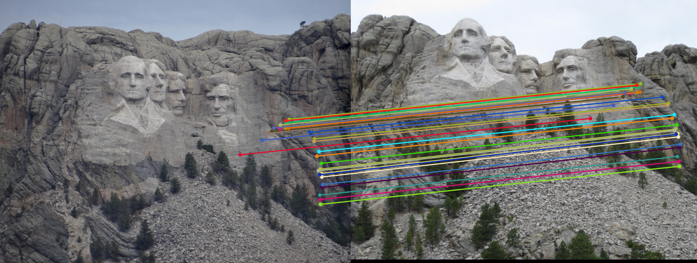
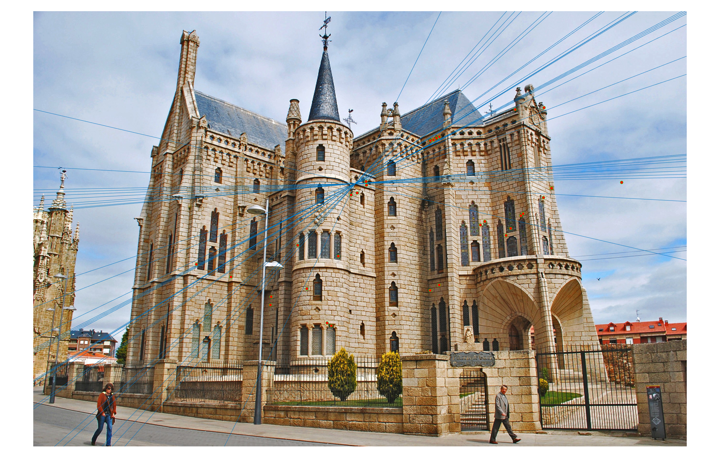
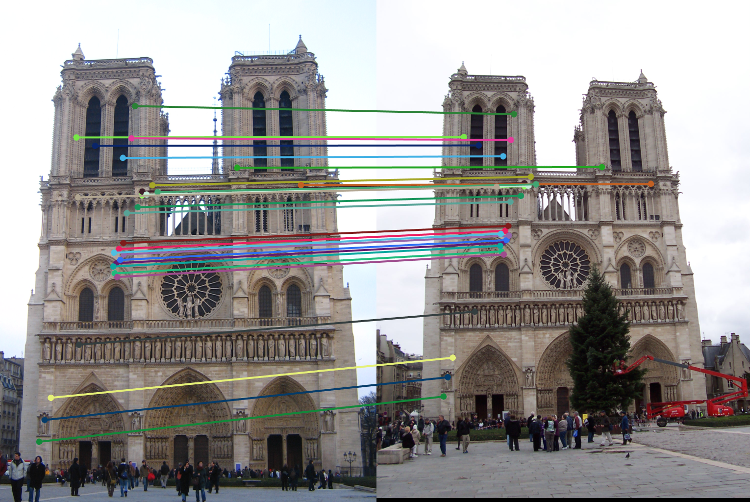
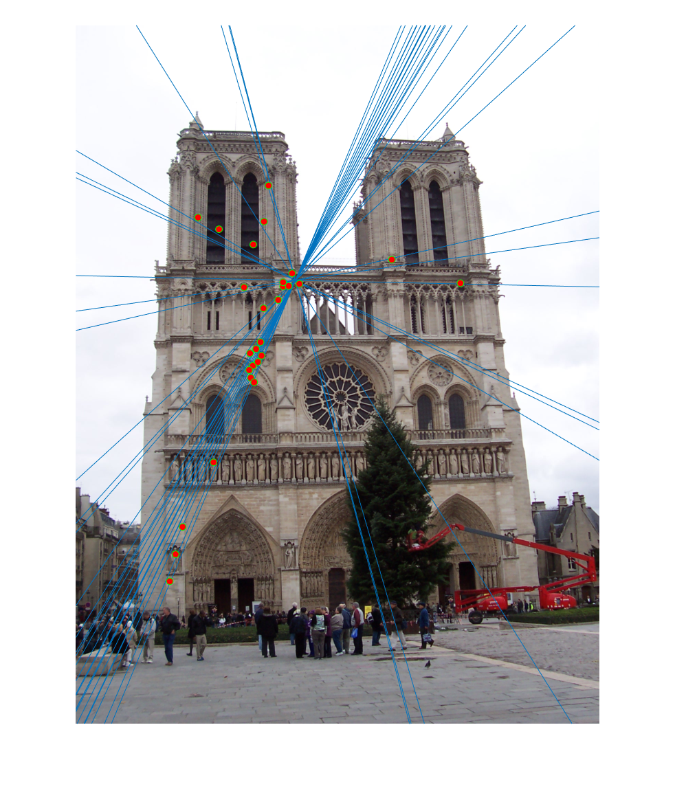
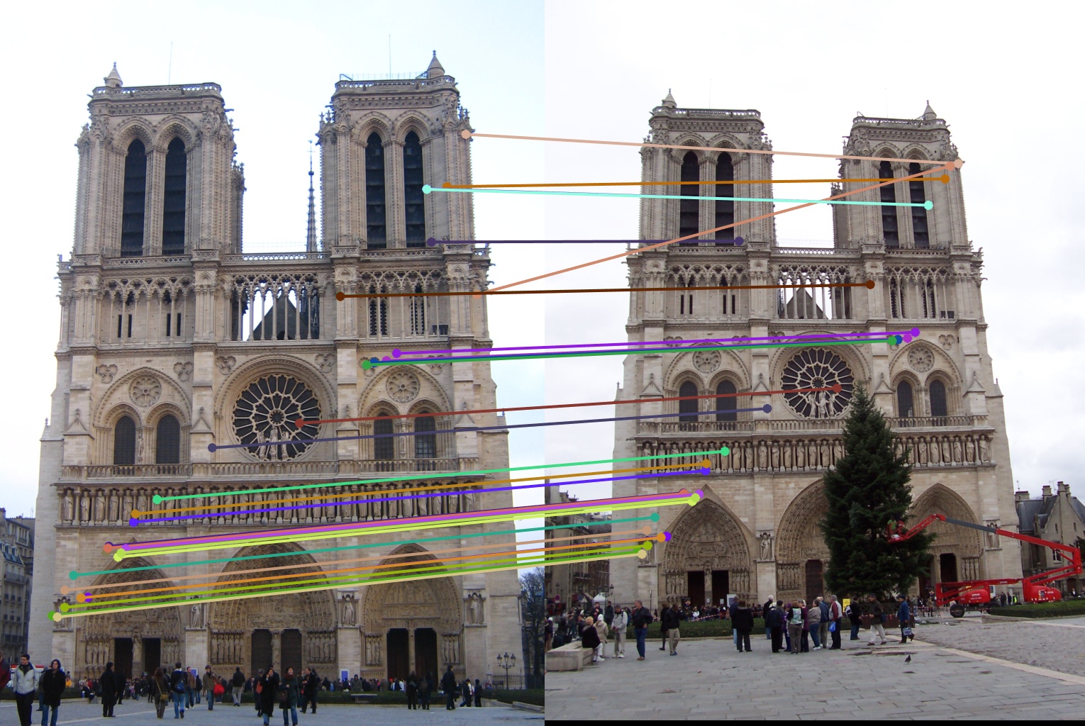
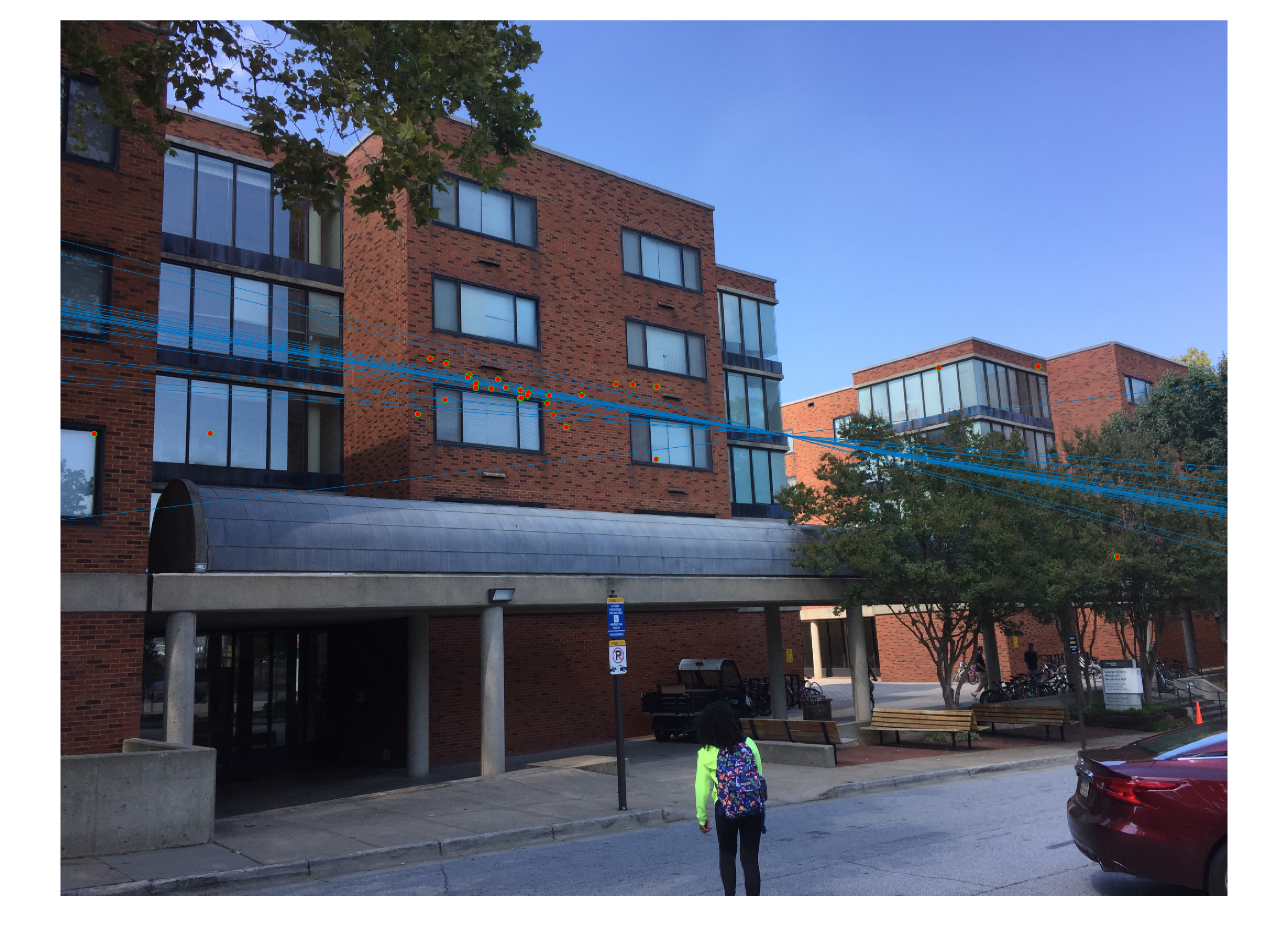
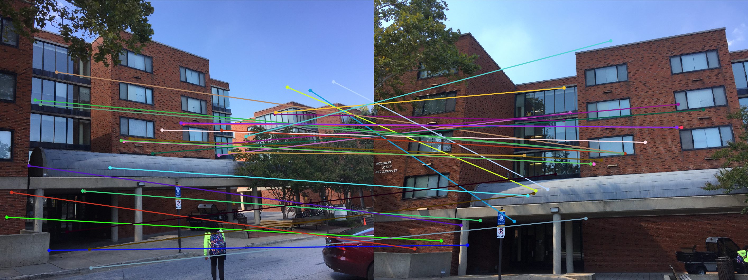
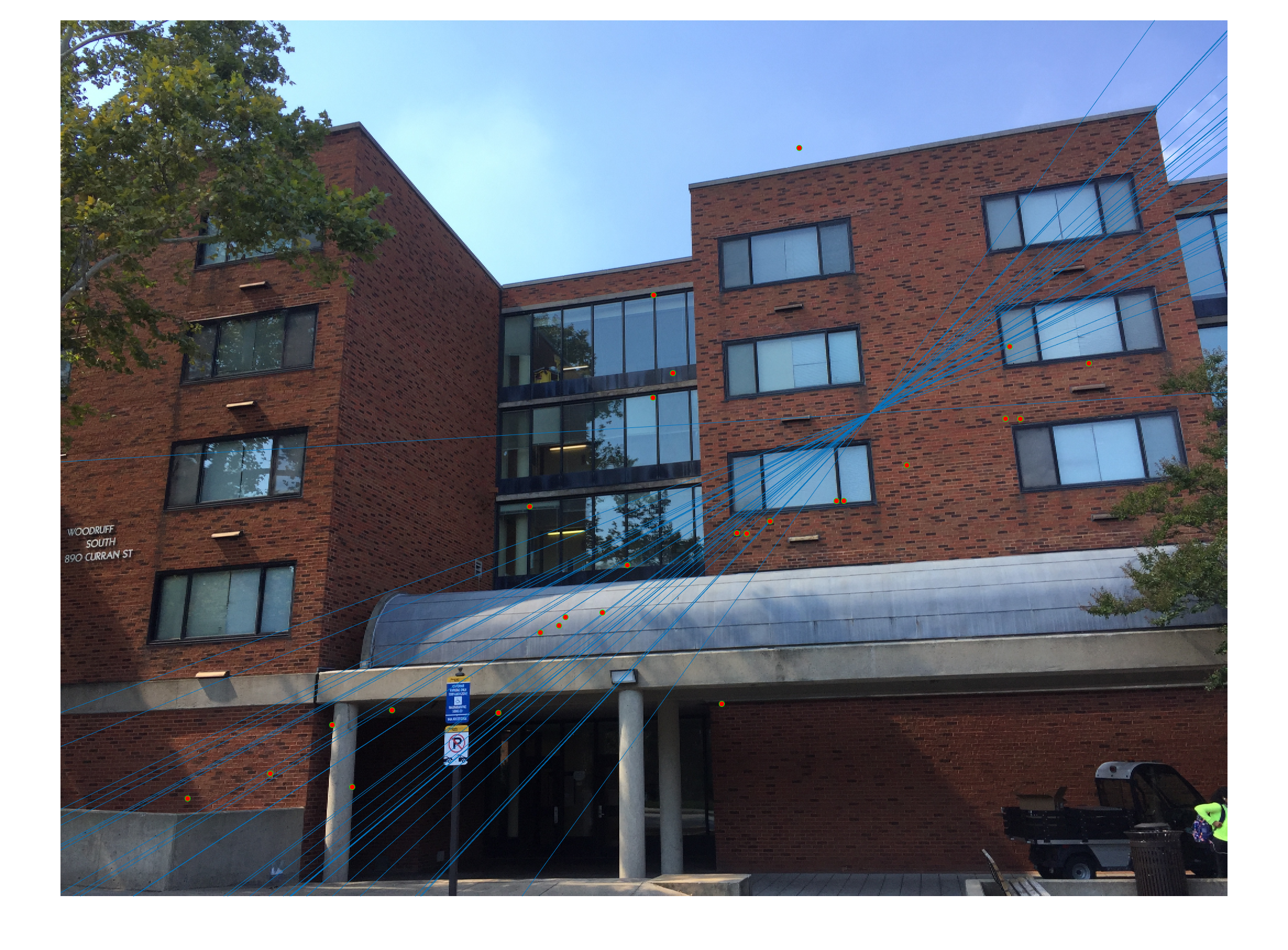
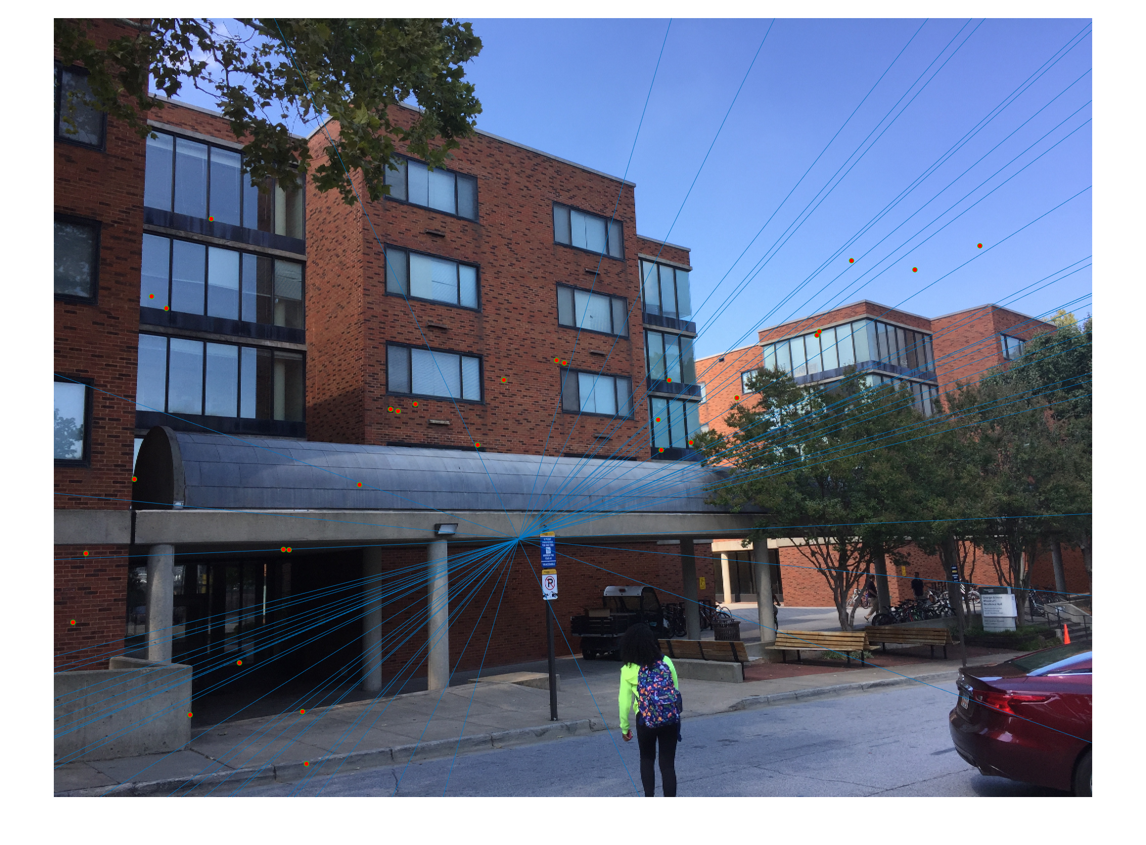
For each pair of rows the first row shows running the algorithm with normalization and the second row shows running without. As can be seen in all the image pairs, the epipolar lines match to the points in both images much better when the fundamental matrix is normalized.