Jingjing Pan

Details

1. Estimate projection matrix

As described in the textbook and the slides, the definition of projection matrix (2D point equals the multiplication of projection matrix and the corresponding 3D point) can be formulated into A * M = 0. In matlab, A can be constructed in this way:

for i=1:n
	r1 = i*2-1;
	r2 = i*2;

	X = Points_3D(i,1);
	Y = Points_3D(i,2);
	Z = Points_3D(i,3);
	u = Points_2D(i,1);
	v = Points_2D(i,2);

	A(r1, 1) = X;
	A(r1, 2) = Y;
	A(r1, 3) = Z;
	A(r1, 4) = 1;
	A(r1, 9) = -u*X;
	A(r1, 10) = -u*Y;
	A(r1, 11) = -u*Z;
	A(r1, 12) = -u;

	A(r2, 5) = X;
	A(r2, 6) = Y;
	A(r2, 7) = Z;
	A(r2, 8) = 1;
	A(r2, 9) = -v*X;
	A(r2, 10) = -v*Y;
	A(r2, 11) = -v*Z;
	A(r2, 12) = -v;

end

where n is the number of matching pairs. The least square solution can be calculated for this homogeneous equation with SVD decomposition:

[U,S,V] = svd(A);
M = V(:,end);
M = reshape(M, [],3)';

Below is the computation result, which agrees with the official solution:

The projection matrix is:
    0.4583   -0.2947   -0.0140    0.0040
   -0.0509   -0.0546   -0.5411   -0.0524
    0.1090    0.1783   -0.0443    0.5968


The total residual is: 0.0445

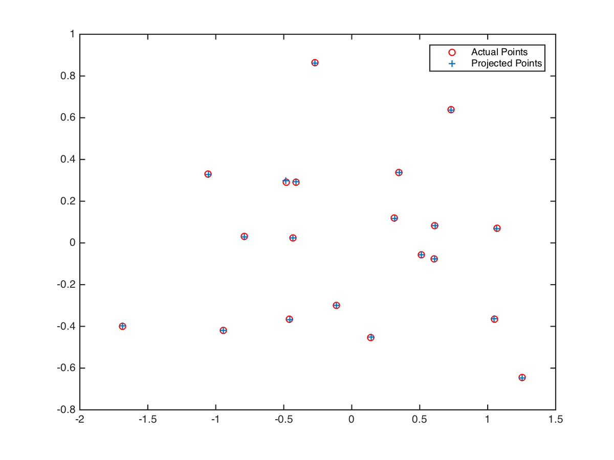
2D visualization of image 2D points and projected 3D points into 2D space gives aligned result:

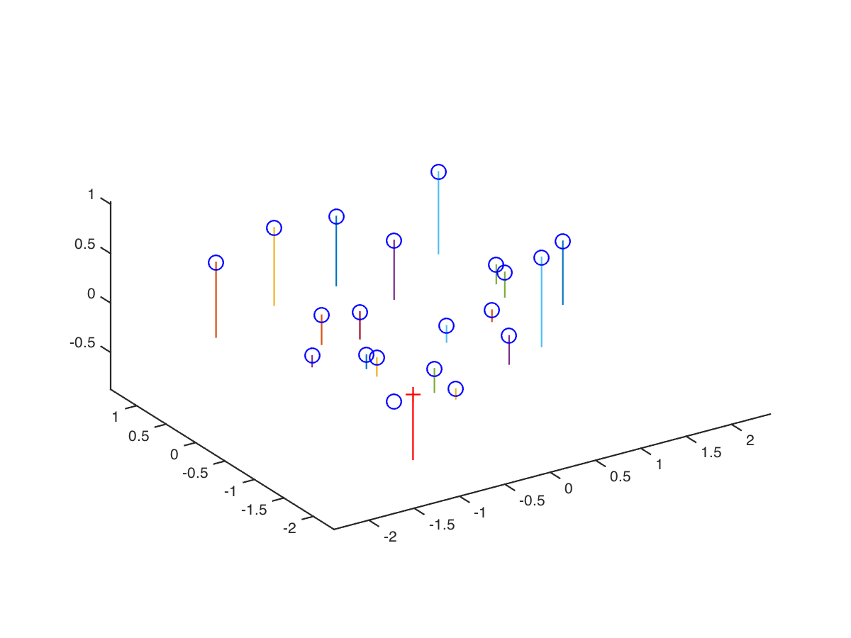
We can further compute camera center with this code and obtain visualization of 3D space below:

Q = M(:, 1:3);
m_4= M(:, 4);
Center = -inv(Q)*m_4;

%% Result:
%% The estimated location of camera is: -1.5127, -2.3517, 0.2826

2. Estimate fundamental matrix

The definition of fundamental matrix (the multiplication of p transpose, F and p' should be zero) can also be transformed into least square problem and then get solved with 8-point algorithm. Code implementation is as below:

for i=1:n
	ua = Points_a(i,1);
	va = Points_a(i,2);
	ub = Points_b(i,1);
	vb = Points_b(i,2);

	A(i, 1) = ua*ub;
	A(i, 2) = ua*vb;
	A(i, 3) = ua;
	A(i, 4) = va*ub;
	A(i, 5) = va*vb;
	A(i, 6) = va;
	A(i, 7) = ub;
	A(i, 8) = vb;
	A(i, 9) = 1;
end

[U,S,V] = svd(A);
f = V(:,end);
F = reshape(f, [3 3]);

The least squares estimate of F is full rank; however, the fundamental matrix is a rank 2 matrix. To reduce the rank of F, we set its last eigenvalue to be zero (and then scale the matrix so that the last entry is 1):

[U,S,V] = svd(F);
S(3,3) = 0;
F = U*S*V';

F_matrix = F;

F_matrix = F_matrix .* (1/F_matrix(3,3));

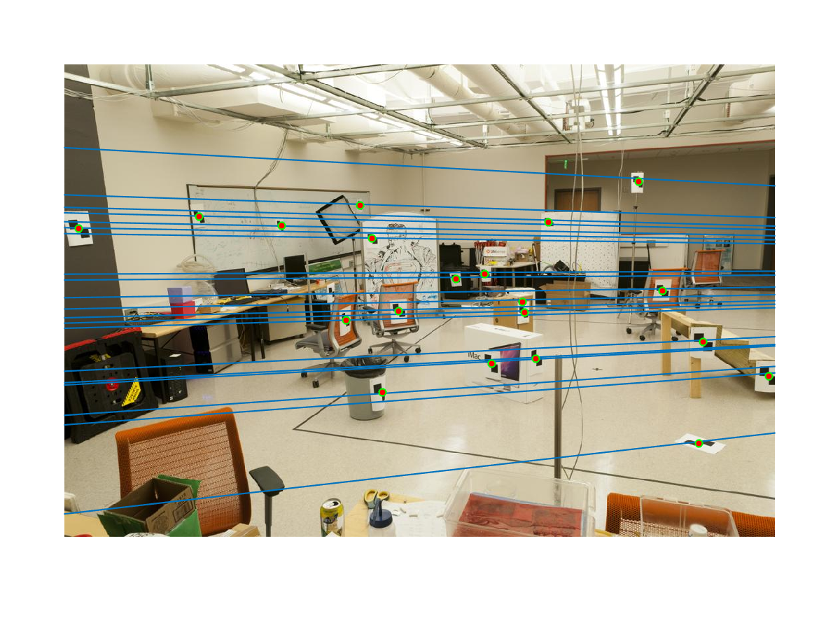
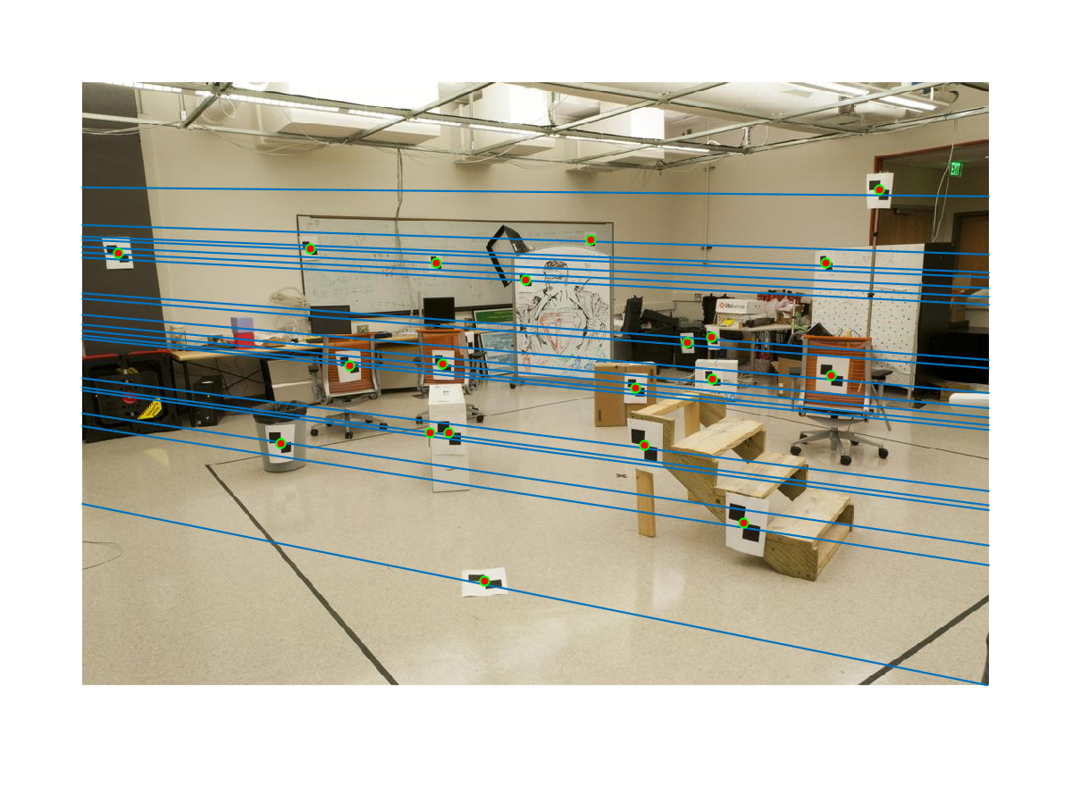
We can obtain this visualization if we draw epipolar lines and the points on the test image pair:

3. Estimate fundamental matrix with SIFT and RANSAC

While we use the same function to estimate fundamental matrix with 8 selected pairs of points, we find the best fundamental matrix with RANSAC since SIFT matching is unreliable. Specificaly, we set parameters of RANSAC as below:

s = 8;
p = 0.99;
e = 0.5;
model_ths = 0.0015;
max_n_inlier = 0;
n_iter = round(log(1-p)/log(1-(1-e)^s)); % n_iter turns out to be 1177

In each iteration, we 1) randomly sample 8 points and 2) estimate fundamental matrix based on the sampled points:

% 1) Randomly sample points
rand_idx = randi(n_pt, 1, s);
matches_a_samp = matches_a(rand_idx, :);
matches_b_samp = matches_b(rand_idx, :);

% 2) Fit model on sampled points
Fmatrix = estimate_fundamental_matrix(matches_a_samp, matches_b_samp);

For the 3rd step of RANSAC, we use the multiplication of matrix A (as defined in part 2) and vectorized F as the distance metric. The reason behind is that p^T*F*p' of a good fundamental matrix estimation and an inlier pair p and p' should have a value very close to zero. If we set a model threshold (0.00015 in this experiment) and count the point pairs that have smaller p^T*F*p' than the threshold and compare the models to find a model with highest number of inliers, then we can say that this model is the most reliable model among the iterations. To make an easier computation of distance matric, we tranform p^T*F*p' into the multiplication of A and F, where A contains point pairs from all SIFT matchings.

% outside the iteration loop:
for i=1:n_pt
	ua = matches_a(i,1);
	va = matches_a(i,2);
	ub = matches_b(i,1);
	vb = matches_b(i,2);

	A(i, 1) = ua*ub;
	A(i, 2) = ua*vb;
	A(i, 3) = ua;
	A(i, 4) = va*ub;
	A(i, 5) = va*vb;
	A(i, 6) = va;
	A(i, 7) = ub;
	A(i, 8) = vb;
	A(i, 9) = 1;
end

% inside the iteration loop, right after 1) and 2):

	% 3) Count inliers
	dist = A*Fmatrix(:); % n_pt x 1
	inlier_idx = find(abs(dist) max_n_inlier
		max_n_inlier = n_inlier;
		Best_Fmatrix = Fmatrix;
		inliers_a = matches_a(inlier_idx,:);
		inliers_b = matches_b(inlier_idx,:);
	end	

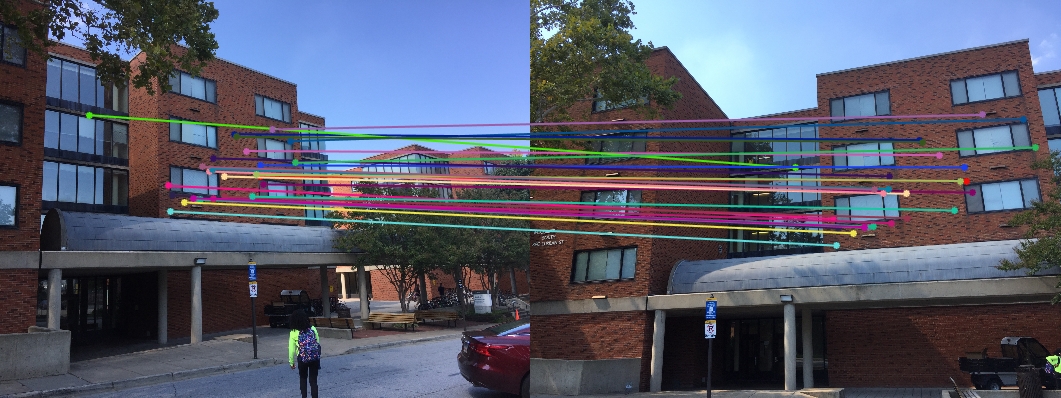
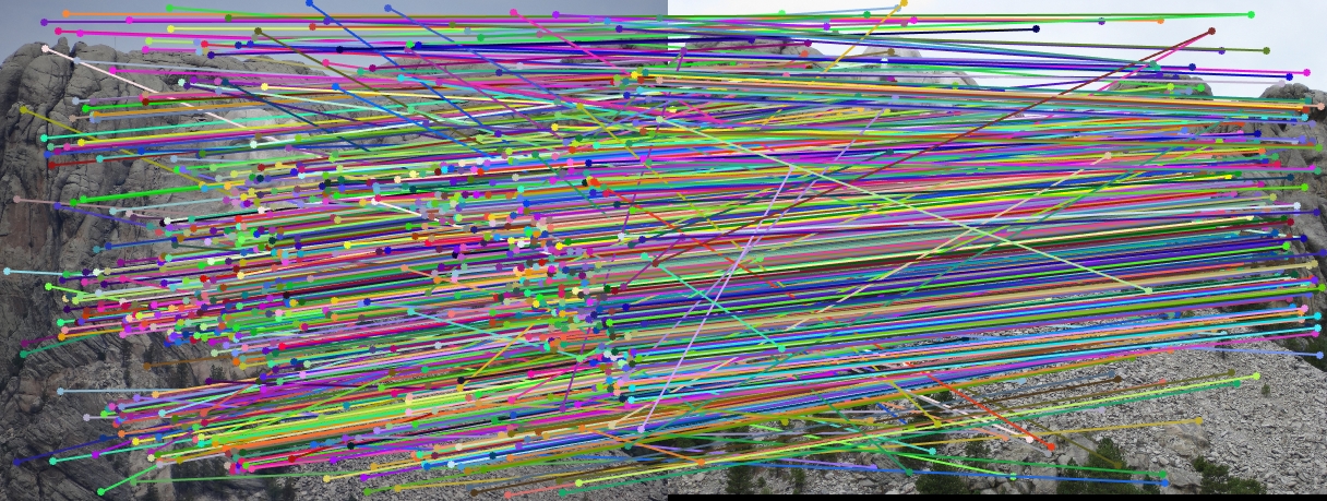
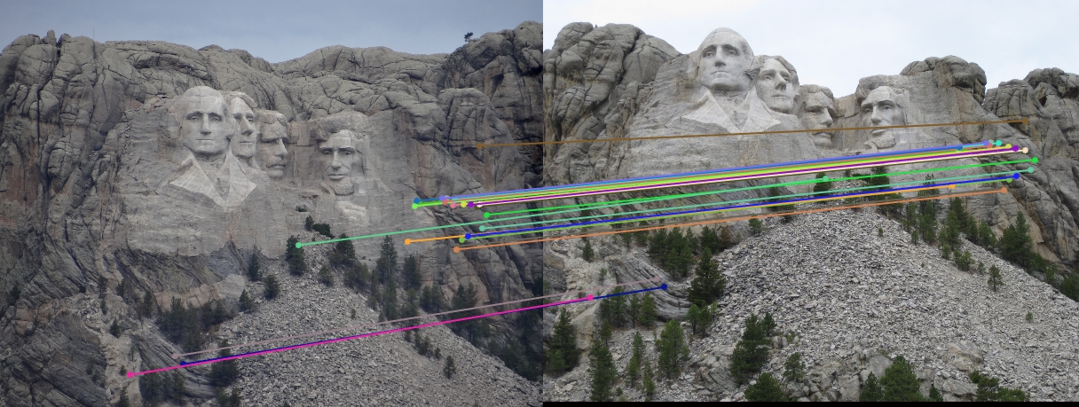
Finally we randomly select 30 inlier pairs to make visualization like this. We did experiments on image pairs of Mount Rushmore, Notre Dame, Gaudi and Woodruff hall. Since I set model threshold to be very low, we found RANSAC did a good job filter out outliers and gives almost only correct matchings. For example, Mount Rushmore has a noisy SIFT matching result (upper), and RANSAC successfully selected true inliers (below):

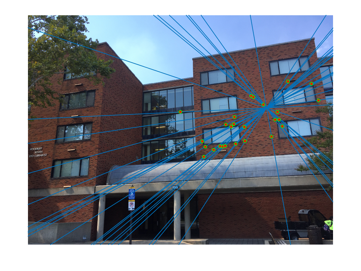
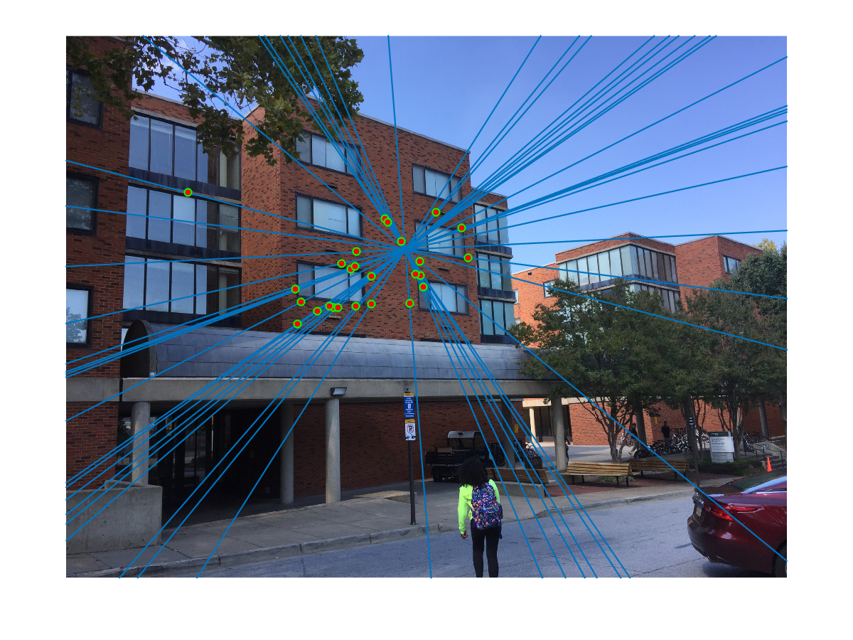
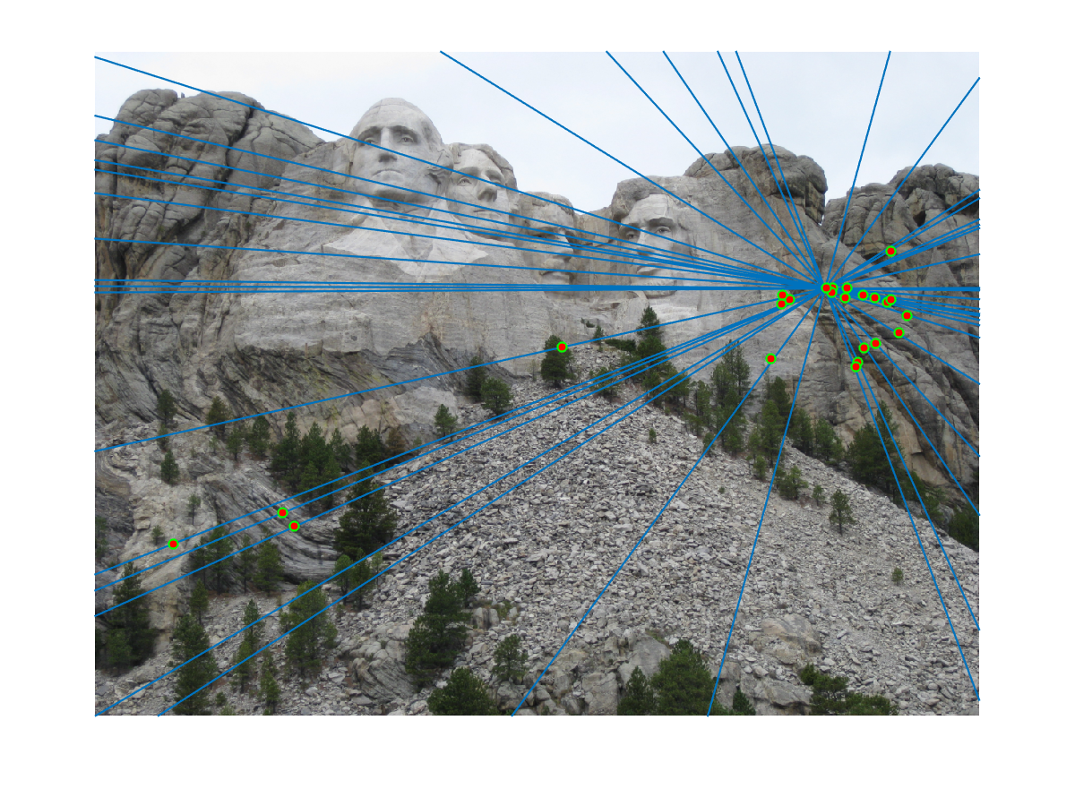
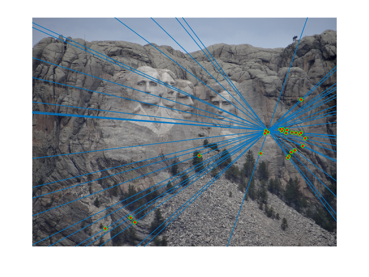
This visualization shows that epipolar lines go through matching points correctly:

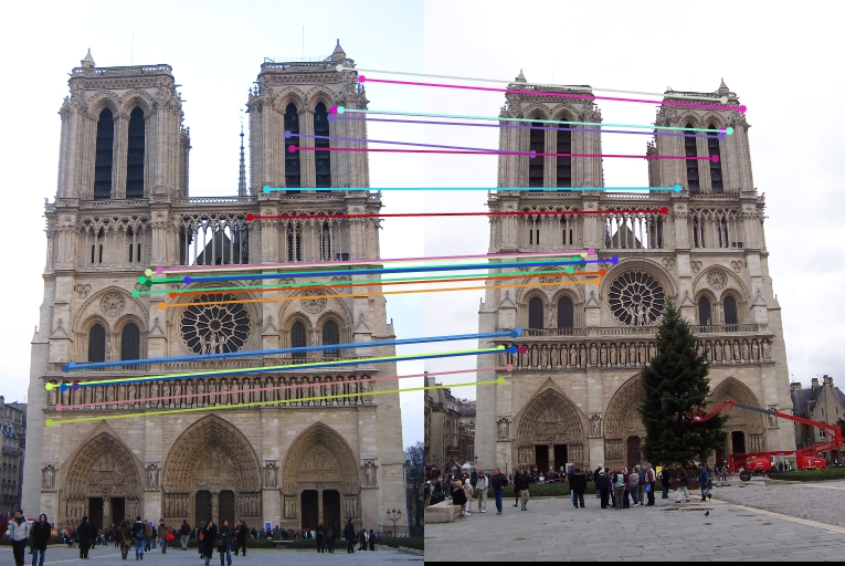
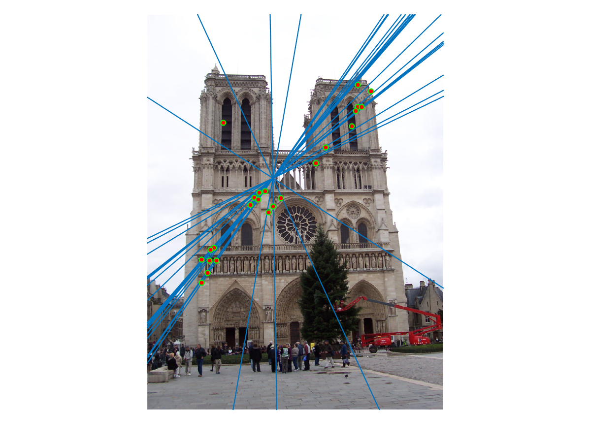
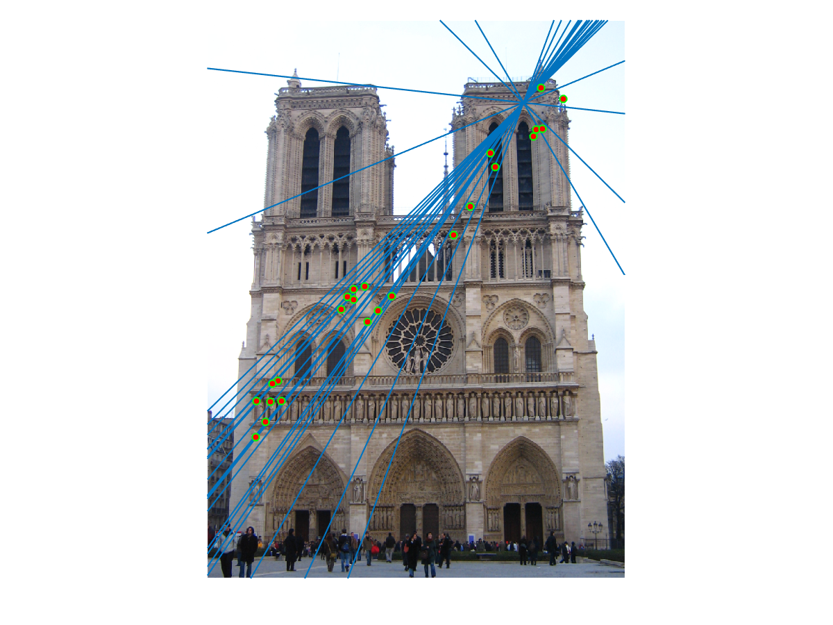
This algorithm works fine with other image pairs. For Notre Dame pair, we use similar visualization to get these results:

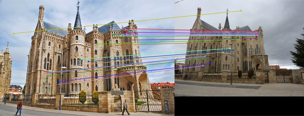
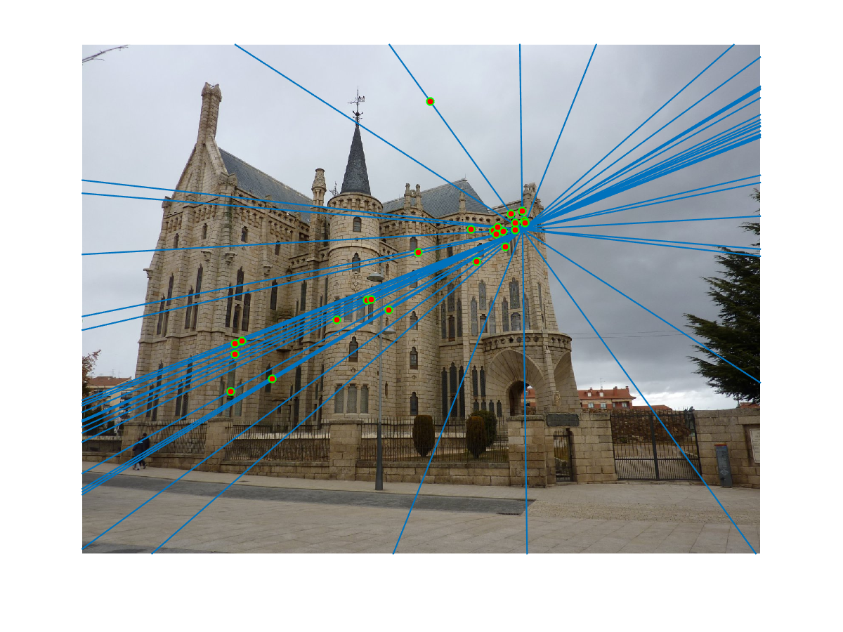
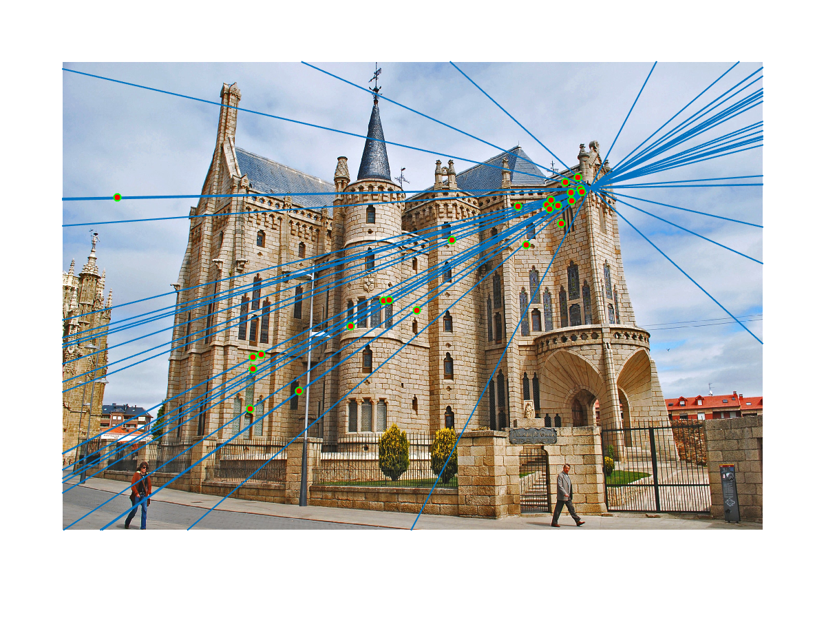
For Gaudi pair:

It also works well with Woodruff pair: