Project 3: Camera Calibration and Fundamental Matrix Estimation with RANSAC
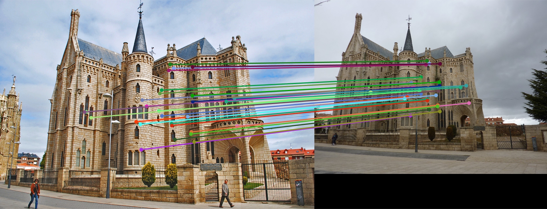
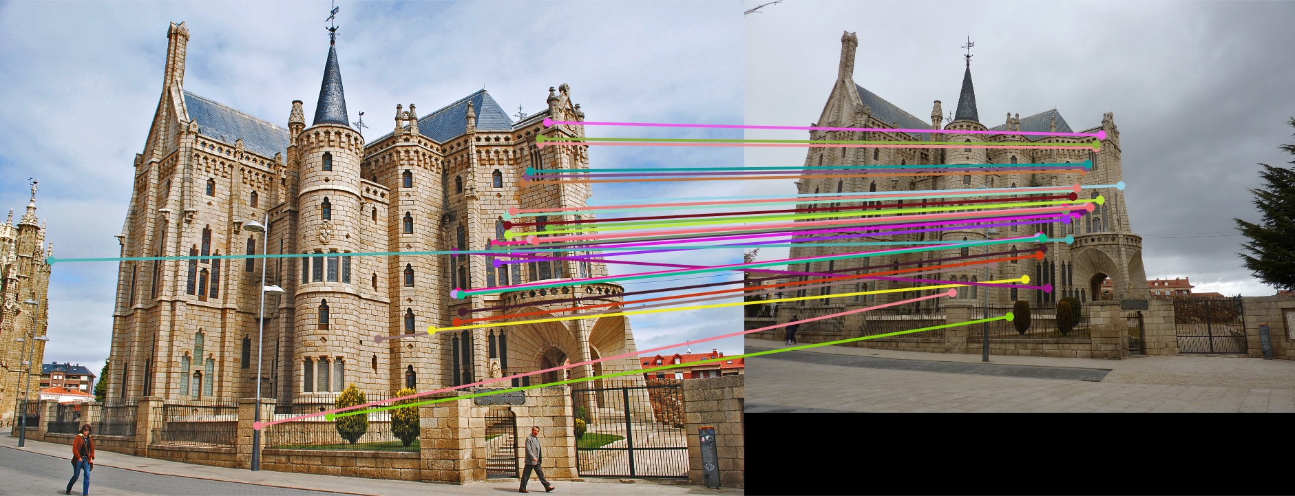
Illustration 1. Point correspondence on a pair of Episcopal Gaudi pictures.
The goal of this project is to become familiar with camera calibration and fundamental matrix estimation. For this purpose, we will work on 3D world coordinates and 2D image coordinates mapping, as well as point correspondence betweeen two images.
The project can be broken down into three main parts:
- Camera Projection Matrix
- Fundamental Matrix Estimation
- Fundamental Matrix Estimation with RANSAC
Let's discuss each of these parts in detail.
1. Camera Projection Matrix
In this part of the project we are provided with 2 sets of points: 1) 2D image coordinates, and 2) 3D world coordinates, and we are asked to calculate the corresponding camera projection matrix that will map both set of points. To do this we will first need set up the a system of equations between the two sets of points. As explained in class,we know that:

Equation 1. Camera projection matrix. Source: CS6476 ppt14.
which can be rewritten as:

Equation 2. Camera projection matrix (II). Source: CS6476 ppt14.
Once that we have set up our system of equations, we are going to use Matlab svd() function to solve the problem. This way, the result we obtain
as our estimation of the projection matrix is as follows:

Equation 3. Camera projection matrix estimation and total residual.
As we can see from the picture, we obtained a total "residual" value of 0.0445, which indicates that the generated matrix maps the two sets of points accurately, with a very small error (total "residual" value: square root of the sum of squared differences in u and v). As it can be seen in Illustrion 3, projected points will match actual points with a slight offset.
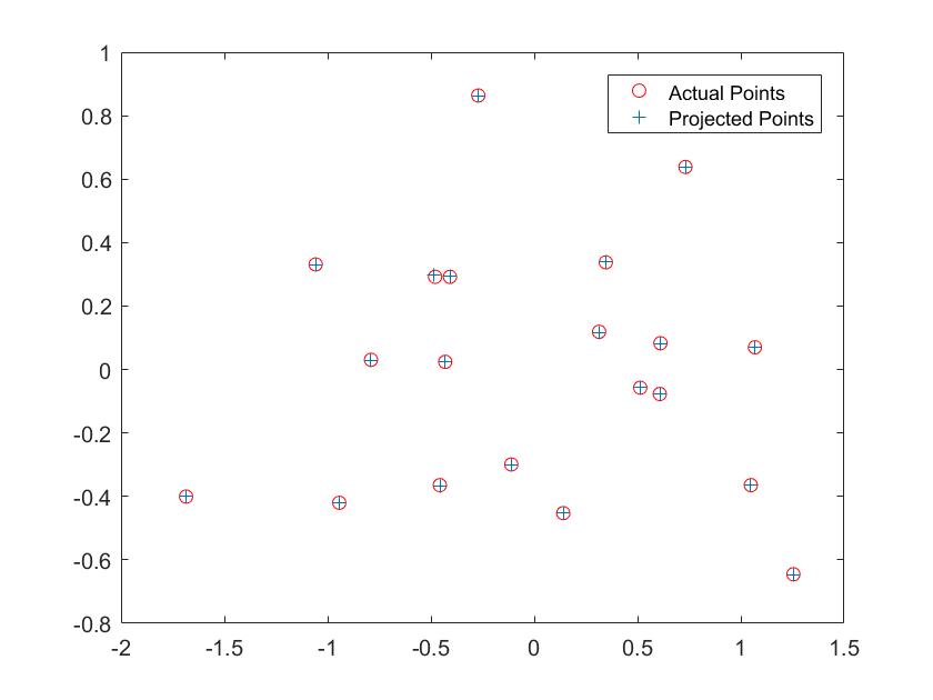
Illustration 3. Actual vs projected points.
It must be noticed that the projection matrix has been calculated using the complete set of points (20), and that a scale factor (-1) has been applied.
Now that we have estimated the camera projection matrix, the next step is to calculate the camera center in world coordinates. For this purpose, we will split the projection matrix M into the instrictic matrix K and the extrinsic matrix [R|t]. As explained in class, we can alternatively have Q = K * R, and m4 = t. This representation turns to be very useful for calculating the camera center, since it can just be written as: C = -Q^(-1) * m4. Thus, only by applying this formula in Matlab we obtained our center estimation:

Illustration 4. Camera center estimation.
2. Fundamental Matrix Estimation
The second part of the project consists in mapping points of two different images of the same scene. This time we are provided with two datasets of 2D points (1 dataset per image), and our goal is to estimate the fundamental matrix. Here we will implement the 8-point algorithm, although we will be using the complete set of points instead of just 8. In this manner, we will set up our system of equations such that:

Equation 4. Fundamental matrix equations.
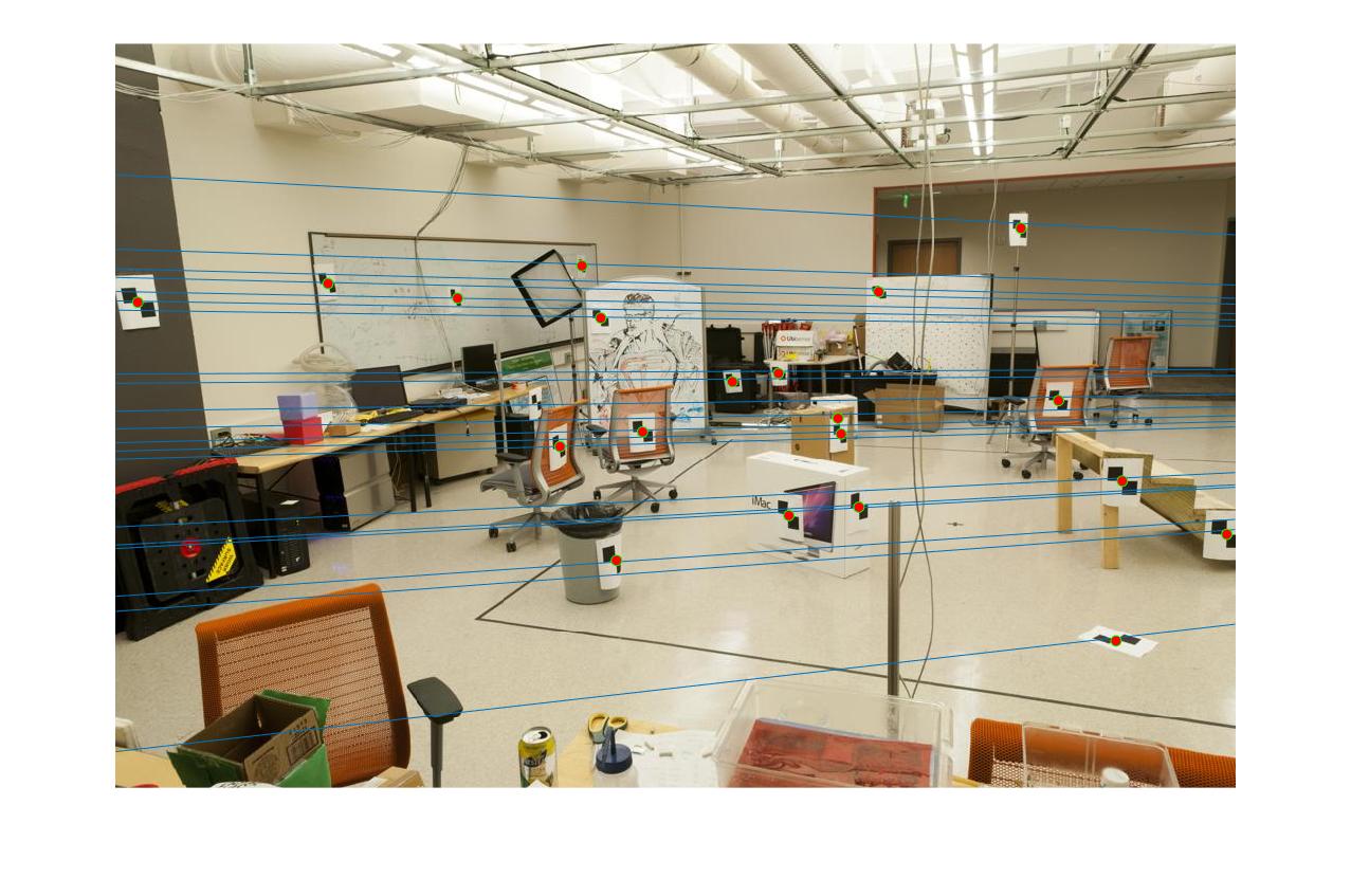
Similarly as part I, we will use svd() function to solve the system of equations, and we will apply rank reduction next. The results obtained are shown in
Illustration 5.

Equation 5. Estimated fundamental matrix values.
|
Illustration 5. Pair of images with their corresponding epipolar lines drawn.
3. Fundamental Matrix Estimation with RANSAC
The goal of this part of the project is the same as the second part. However, this time instead of receiving ground truth point correspondences, we will receive them in a more realistic manner, more exactly, these correspondences of points will be obtained from SIFT algorithm. This means that, since the point correspondences are less reliable now, we should implement a method robust to noisy data. For this purpose, we will use RANSAC and our function developed in part II to estimate the fundamental matrix.
The idea behind applying RANSAC in conjunction with part II, is that here we will create different models using 8 random points (minimun number of points to solve the equations) each time, and compute their estimated fundamental matrixes, but we will only keep the fundamental matrix that obtains the best result. Now how can we determine which matrix work best? For that purpose we will use a metric that will count the number of pair of points (inliers) that 'agree' with each fundamental matrix, and select the one that returns the highest value. As we can see, there are two main parameters that can be adjusted in this model: number of iterations, and threshold. As the number of iterations increases the more refined our result will be, since more submodels have been considered, but the higher the running time will be as well. Similarly for the threshold, we want a value that will reject incorrect matches, but will keep as many as correct matches as possible.
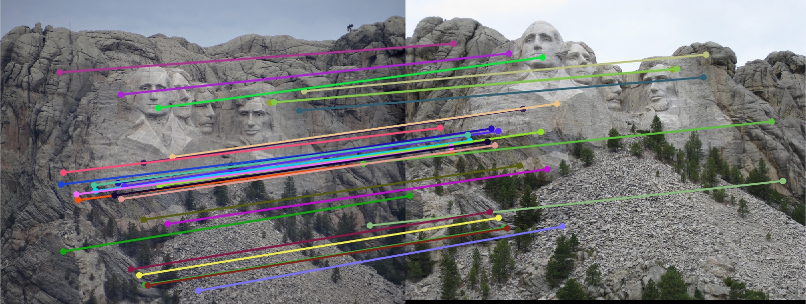
Here are some of the results obtained: * images show the 30 best inliers, i.e. pairs of point with the lowest distance error.
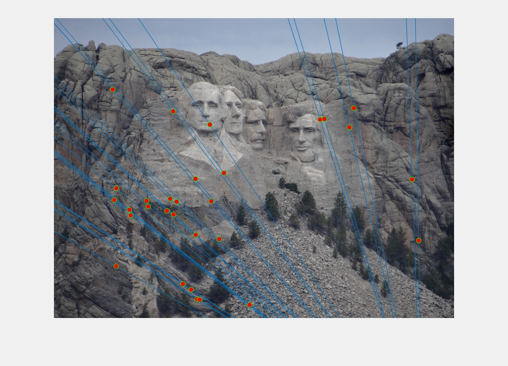
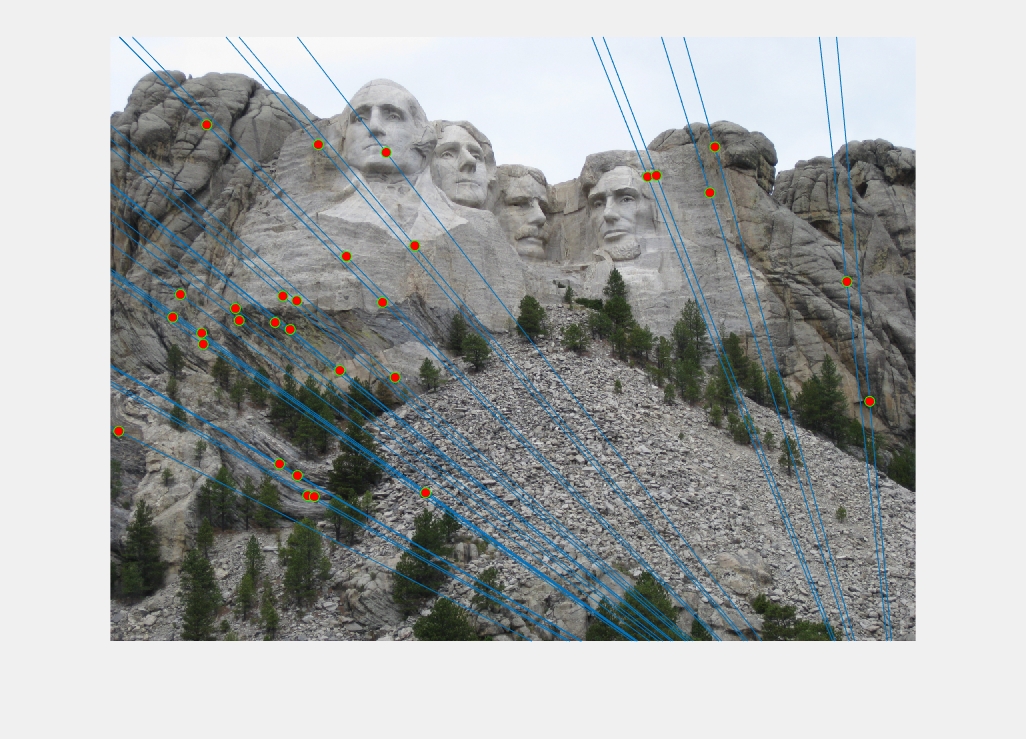
Mountain Rushmore: iterations: 2000, threshold: 0.05
|
Illustration 5. Epipolar lines drawn on Mountain Rushmore pair of images.
This configuration gives us a high number of inliers: 603. Although I could have decreased the threshold to limit this number, I think that the correspondences shown are mainly correct.
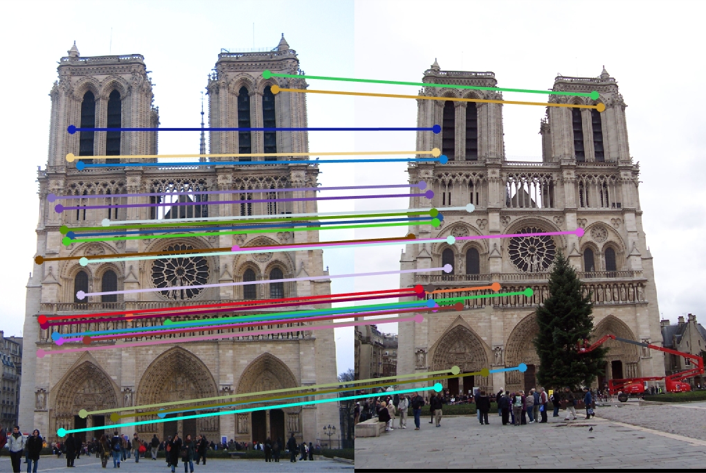
Notre Dame: iterations: 2000, threshold: 0.05
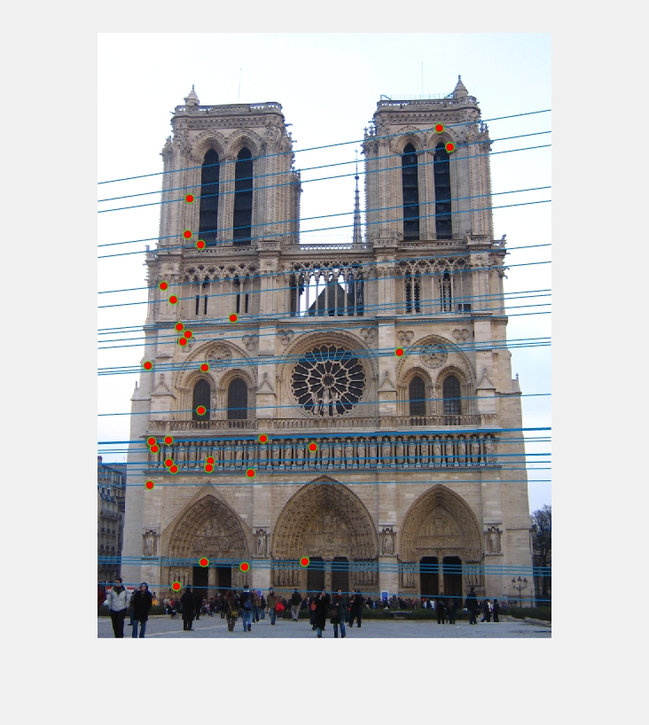
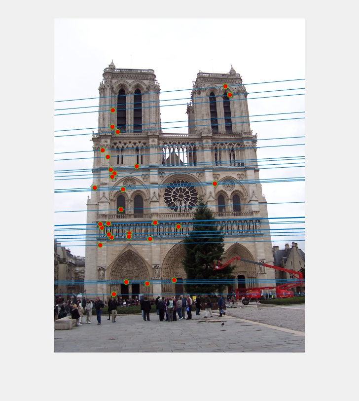
|
Illustration 6. Epipolar lines drawn on Notre Dame pair of images.
The configuration for this image is the same as for Mountain Rushmore, and we can observe from the picture that the accuracy is good as well. This time we got 538 inliers.
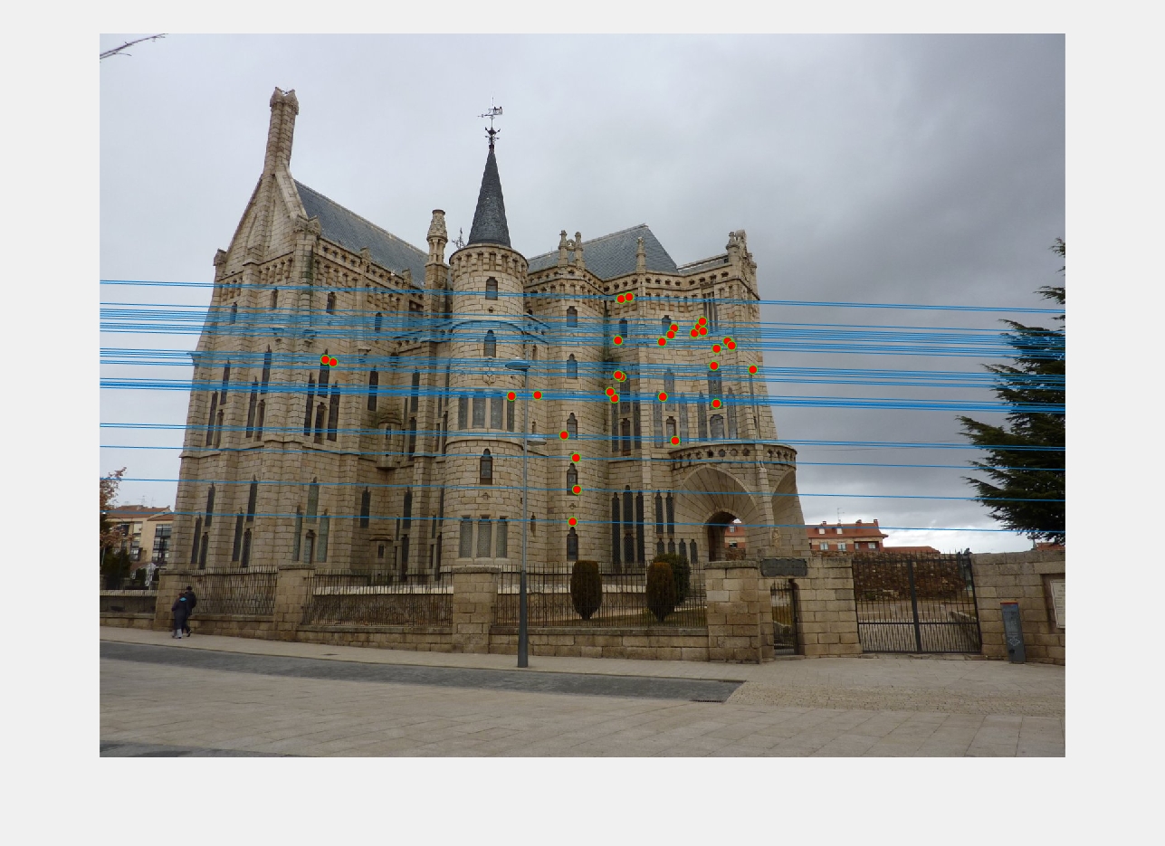
Episcopal Gaudi: iterations: 10000, threshold: 0.005
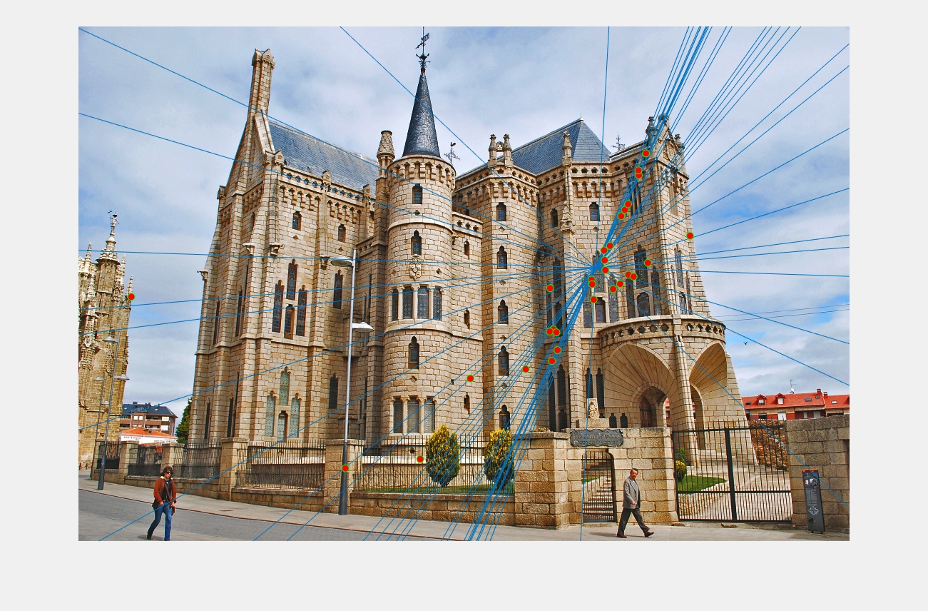
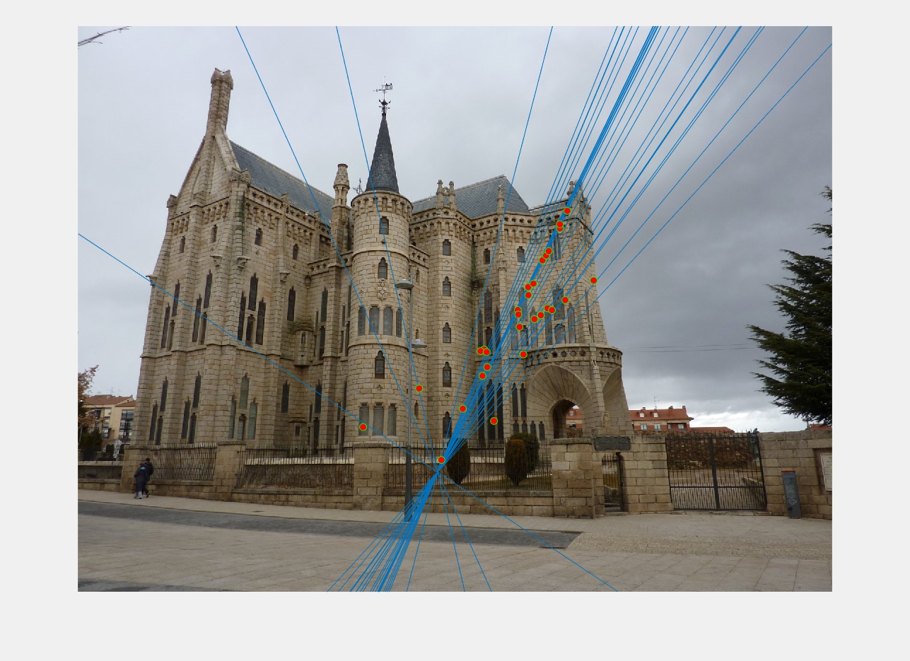
|
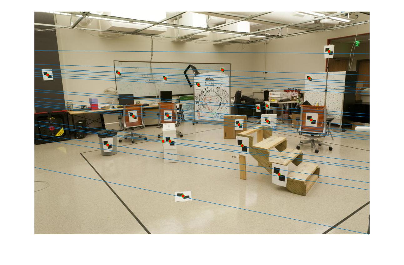
Illustration 7. Epipolar lines drawn on Episcopal Gaudi pair of images.
We were stricter with the configuration of this pair of images. Because of the images characteristics, finding the correspondence between these points becomes harder. This time, we set number of iterations to 10000 (so that more models were being tested) and threshold to 0.005 (we are being more conservative about what to consider an inlier). This time our number of inliers dropped to 200.
As we can see, this implementation does not work for every pair of images. For some of them normalization is required to achieve good correspondences.
4. Extra credit/Normalization
In this section we will improve our fundamental estimation by normalizing input images coordinates. To this end, we implemented the following steps:
- Calculate T matrixes, and normalize each pair of points
Since T is the product of the scale and offset matrices, we needed to compute the scale and the mean for each image. For the scale value, we decided it to be such that the average squared distance for every point will be 2 (after translating them using mean values).
- Select "best" fundamental matrix
This will be done by calling estimate_fundamental_matrix iteratively, and passing the normalized points as input.
- Return best fundamental matrix and inliers
Here we will transform the best fundamental matrix so that it can be applied to the original images. We will do this by using T matrixes (Ta and Tb). For the matches, we actually do not need to transform the values, the way I implemented the algorithm I just needed to know their corresponding indexes in the scaled matrixes.
I decided to normalize points sets as a whole instead of computing the normalization for only the eight points used in each turn, because this way seemed less biased to me. Also, normalizing in each iteration would require a longer running time. In the same way, I decided to only transform matrixes to the original scale once the final fundamental matrix was found.
Here is the result for Episcopal Gaudi. As we can see, point correspondences are much more accurate here than in the previous pair of images without normalization. Also it must be noticed than we decreased the number of iterations from 5000 to 2000, and increased the threshold from 0.005 to 0.05. The number of inliers for the 'best' matrix is 544.
Episcopal Gaudi (with normalization): iterations: 2000, threshold: 0.05
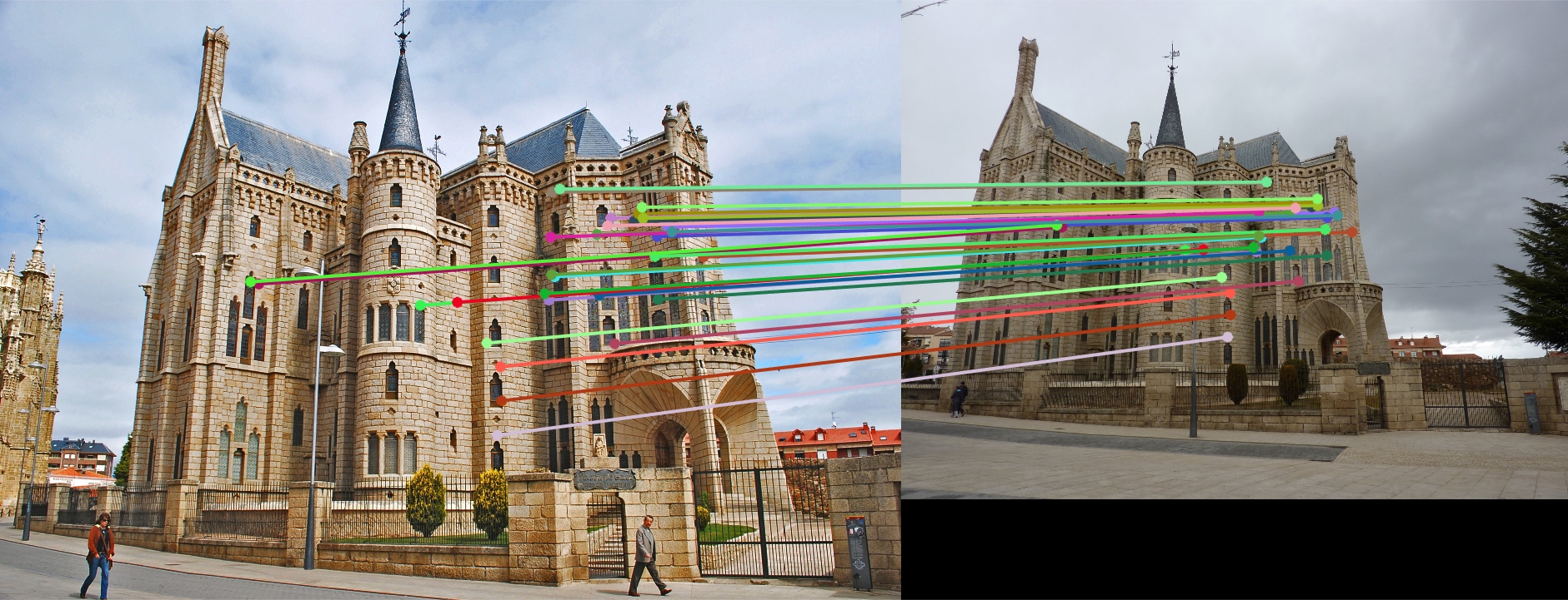
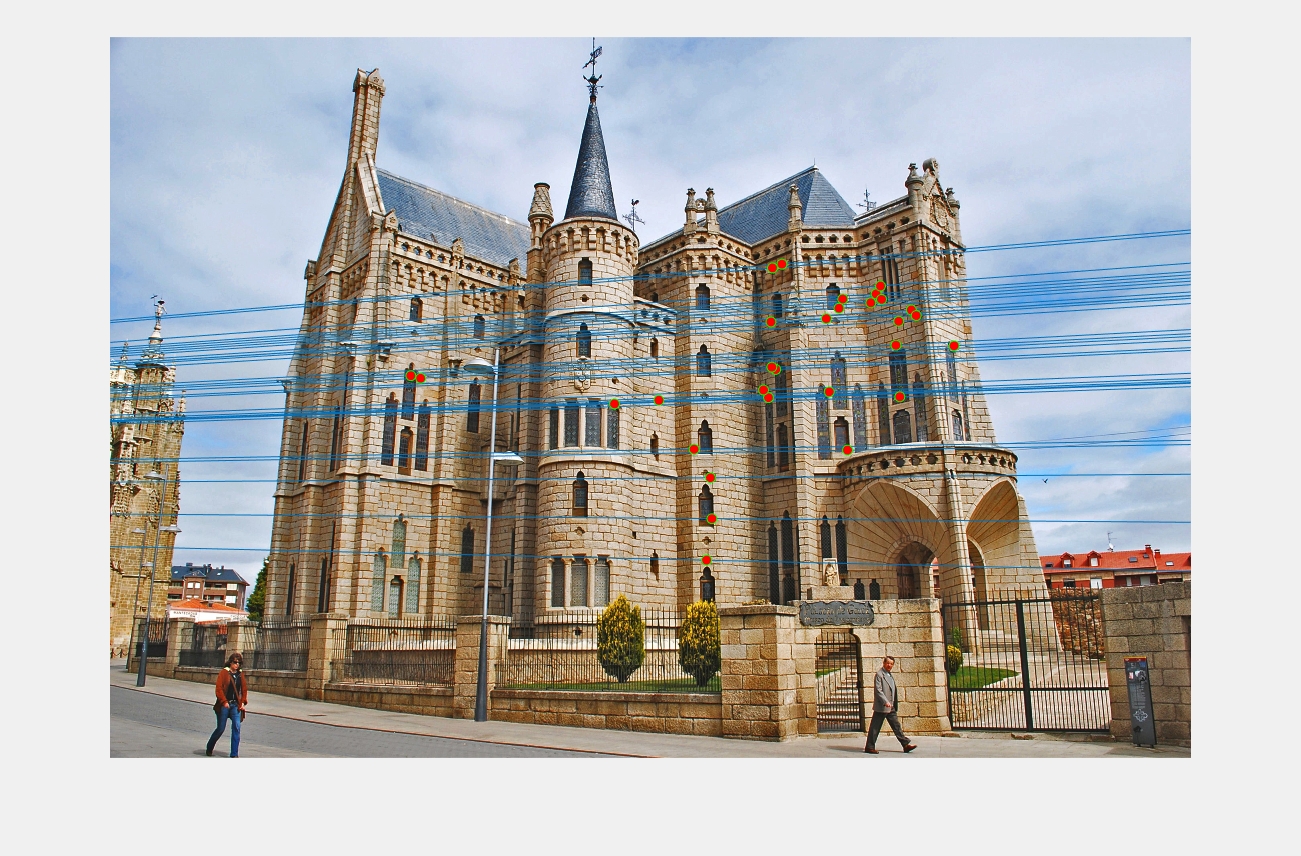
|
Illustration 8. Epipolar lines drawn on Episcopal Gaudi pair of images (with normalization).