Kshitish Deo

Project 2: Local Feature Matching

This project covers camera caliberation, creating robust fundamental matrix and implementing RANSAC. We calculate the projection matrix with which we get the camera center in the fisrt part. Second part focuses on finding fundamental matrix. In this part normalization is covered to get robust fundamental matrix. Inliers are seperated from the outliers by using RANSAC algorithm.

There are following parts in the project.

1. Camera Caliberation
2. Fundamental Matrix and epipolar lines
3. Ransac method
4. Improved fundamental matrix by normalized coordinates
5. Analysis before and after normalization
6. Results with different images

Camera Caliberation

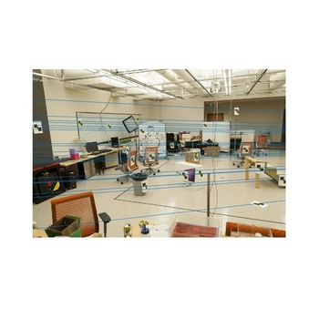
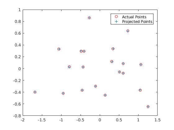
The basic task here is to find 2D coordinates from 3D coordinates given. We get linear regression equation from 2D and 3D points. It is of form 2D_points= M*3D_points. Here M is the projection matrix.But there is a problem in this. The matrix M is for a perticular scale. To overcome this part, we fix the last element M(3,4) to 1. Thus following projection matrix is obtained which is exactly similar to the estimated projection matrix in the project description.The residual distance obtained is :0.0445

Following is the projection matrix:

                                               

-0.4583	0.2947	0.0140	-0.0040
0.0509	0.0546	0.5411	0.0524
-0.1090	-0.1783	0.0443	-0.5968

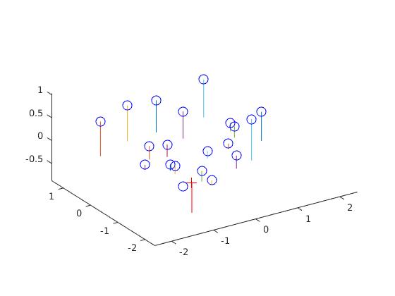
After getting the projection matrix we can get the camera center. The equation: C = -(Q^-1) x (m_4)

We get the above equation from M = (Q | m_4 ). Here C is the camera center. We have taken Q as 3x3 matrix and m_4 is the forth column.

The camera center obtained is = <-1.5127, -2.3517, 0.2826>.

Code for projection matrix

%Getting projection matrix:

%Writing equation in linear form
A(:,1)=Points_3D(:,1);
A(:,2)=Points_3D(:,2);
A(:,3)=Points_3D(:,3);
A(:,4)=1;
A(:,11)= -(Points_2D(:,1).*Points_3D(:,3));
A(:,10)= -(Points_2D(:,1).*Points_3D(:,2));
A(:,9)= -(Points_2D(:,1).*Points_3D(:,1));
A(:,12)=- Points_2D(:,1);
B(:,5)=Points_3D(:,1);
B(:,6)=Points_3D(:,2);
B(:,7)=Points_3D(:,3);
B(:,8)=1;
B(:,11)= -(Points_2D(:,2).*Points_3D(:,3));
B(:,10)= -(Points_2D(:,2).*Points_3D(:,2));
B(:,9)= -(Points_2D(:,2).*Points_3D(:,1));
B(:,12)=- Points_2D(:,2);
X(1:2:end,:) = A;
X(2:2:end,:) = B;
%The above is homogenous equation
[U, S , V]= svd(X);
M= V(:, end);
M
M = reshape(M,[],3)';
M=-M;
M

Code for camera center

M1= M(:,1:3)
M2=M(:, 4)
%writing in form C = -(Q^-1) x (m_4)
Center=-inv(M1)*M2;

RESULTS 1

Fundamental Matrix and epipolar lines

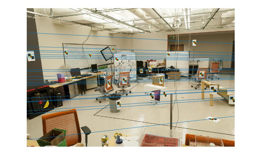
The second part involves finding fundamental matrix and drawing epipolar lines. Fundamental matrix is used for estimating the points for mapping in one image to lines in another.There are one equation per point. We start getting regression lines like above with 9 unknown points. Similarly, we can solve by 8 point algorithm. The last one is fixed to scale the matrix.

The fundamental matrix should be of rank 2. So we decompose F using singular value decomposition into the matrices U ΣV' = F. Then we get 2 matrix by setting the smallest singular value in Σ to zero.

The fundamental matrix is =

                                               

-0.0000	0.0000	-0.0019
0.0000	0.0000	0.0172
-0.0009	-0.0264	0.9995

Code for fundamental matrix

[x_a,y_a]=size(Points_a);
[x_b,y_b]=size(Points_b);

u= Points_a(:,1);
v= Points_a(:,2);
u1= Points_b(:,1);
v1= Points_b(:,2);

%creating linear equation
M=zeros(x_a,9 );
M(:,1)=u.*u1;
M(:,2)=u.*v1;
M(:,3)=u;
M(:,4)=v.*u1;
M(:,5)=v.*v1;
M(:,6)=v;
M(:,7)=u1;
M(:,8)=v1;
M(:,9)=ones(x_a,1);

[U, S, V] = svd(M);
f = V(:, end);
f=f';
F = reshape(f, [3 3]);
%k = rank(F_matrix)
% output of k is 2
[U, S, V] = svd(F);
S(3,3) = 0;
F_matrix = U*S*V';
F_matrix(isnan(F_matrix))=0;

RESULTS 2

RANSAC

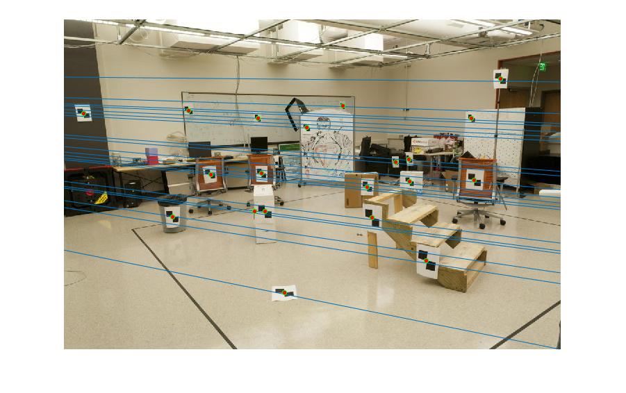
RANSAC is used for best fundamental matrix by removing the outliers. We need to iteratively choose some points (10 in the code), and call estimate_fundamental matrix code to get the fundamental matrix for that point. Here we count the number of inliers. The linear eqaution from the estimated inliers should result in value close to one. In the code the value is fixed to 0.005 which acts as threshold between the inliers and the outliers.

The best fundamental matrix is for one of the trial run was=

                                               

-0.0000	0.0000	0.0081
0.0000	0.0000	-0.0152
-0.0065	0.0122	-0.9998

Code for ransac function

%ransac function
iterations=1000;    % iterations
[x_match,y_match]=size(matches_a);
best=0;
iteration_number=0;
for i=1: iterations
    rand_num=randsample(x_match,10)
    m_a =matches_a(rand_num,:);
    m_b =matches_b(rand_num,:);
    f_matrix= estimate_fundamental_matrix(m_a,m_b);
    [flag, inliers_a1 , inliers_b1]=test_inliers1(f_matrix,matches_a,matches_b); % seperate funtion!
    if (flag==0)
        continue;
    end    
    if best< size(inliers_a1,1)
        Best_Fmatrix=f_matrix;     
        inliers_a=inliers_a1;
        inliers_b=inliers_b1;    
        best=size(inliers_a,1);
        iteration_number=i;
    end

end

Code for test_inlier function

    flag=0;
    M=M';
    M=reshape(M,9,1);
    [x_a,y_a]=size(matches_a);
    [x_b,y_b]=size(matches_b);

    u= matches_a(:,1);
    v= matches_a(:,2);
    u1= matches_b(:,1);
    v1= matches_b(:,2);

    M1=zeros(x_a,9 );
    
    M1(:,1)=u.*u1*M(1,1);
    M1(:,2)=u1.*v*M(2,1);
    M1(:,3)=u1*M(3,1);
    M1(:,4)=v1.*u*M(4,1);
    M1(:,5)=v.*v1*M(5,1);
    M1(:,6)=v1*M(6,1);
    M1(:,7)=u*M(7,1);
    M1(:,8)=v*M(8,1);
    M1(:,9)=ones(x_a,1)*M(9,1);
    
    sum_matrix=sum(M1,2);
    [sum_x,sum_y]=size(sum_matrix);
    b=find(sum_matrix<0.005 &  sum_matrix> -0.005);    %threshold
    disp('size of b')
    [b_x,b_y]=size(b)
    if b_x  == 0
        flag=0;
        inliers_a=[];
        inliers_b=[];
    else        
        flag=1;
        inliers_a=matches_a(b,:);
        inliers_b=matches_b(b,:);
    end
end

RESULTS 2

Normalized coordinates for fundamental matrix

In the third part, normalization of coordinates is done. Translation is done to get the mean at the center. And scaling is done by reducing the image to standard deviation.

A=SxTxA_original

And we get back the original fundamental matrix by F_o=Tb' x F x Ta

Code for test_inlier function

mu=mean(u);
u_1=u-(mu*ones(size(u)));
su=std(u_1);
isu=1./su;
mv=mean(v);
v_1=v-(mv*ones(size(v)));
sv=std(v_1);
isv=1./sv;


mu1=mean(u1);
u_2=u1-mu1*(ones(size(u1)));
su1=std(u_2);
isu1=1./su1;

mv1=mean(v1);
v_2=v1-mv1*(ones(size(v1)));
sv1=std(v_2);
isv1=1./sv1;


% for u,v
scalingM=[isu,0,0;0,isv,0;0,0,1];
transM=[1,0,-mu; 0,1, -mv; 0,0,1];
mod_u=zeros(size(u));
mod_v=zeros(size(v));
one=ones(size(u));
T=scalingM*transM;   %for first T

mod_u=T(1,1)*u+T(1,2)*v+T(1,3)*one;
mod_v=T(2,1)*u+T(2,2)*v+T(2,3)*one;



% for u1,v1
scalingM1=[isu1,0,0;0,isv1,0;0,0,1];
transM1=[1,0,-mu1; 0,1, -mv1; 0,0,1];
T11=scalingM1*transM1;  %for second T
mod_u1=T11(1,1)*u1+T11(1,2)*v1+T11(1,3)*one;
mod_v1=T11(2,1)*u1+T11(2,2)*v1+T11(2,3)*one;



M(:,1)=mod_u.*mod_u1;
M(:,2)=mod_u.*mod_v1;
M(:,3)=mod_u;
M(:,4)=mod_v.*mod_u1;
M(:,5)=mod_v.*mod_v1;
M(:,6)=mod_v;
M(:,7)=mod_u1;
M(:,8)=mod_v1;
M(:,9)=ones(x_a,1);
[U, S, V] = svd(M);
f = V(:, end);
f=f';
F = reshape(f, [3 3]);


[U, S, V] = svd(F);
S(3,3) = 0;
%V = V(:, end);
V=V';
F_matrix1 = U*S*V;


T11=T11';
F_matrix=T11*F_matrix1*T
k = rank(F_matrix);
F_matrix(isnan(F_matrix))=0;

RESULTS 4

ANALYSIS

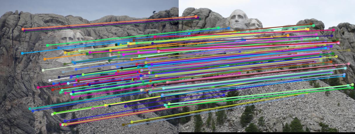
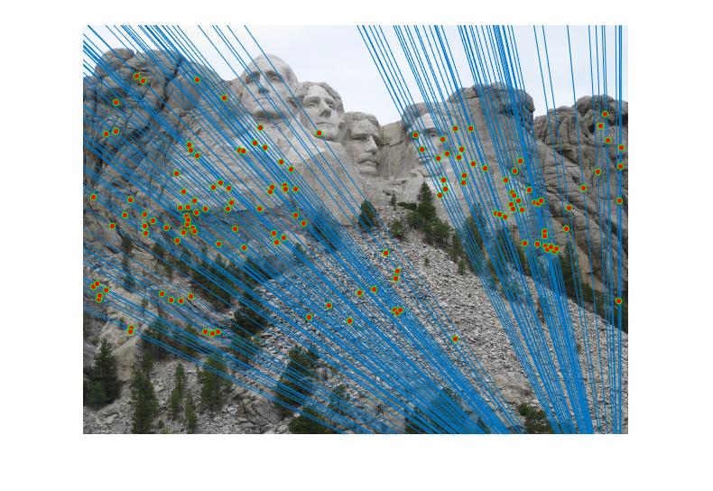
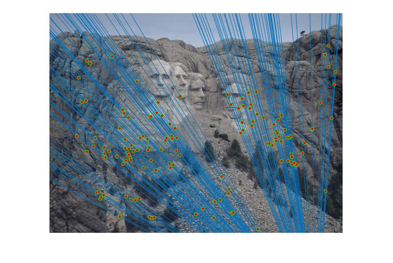
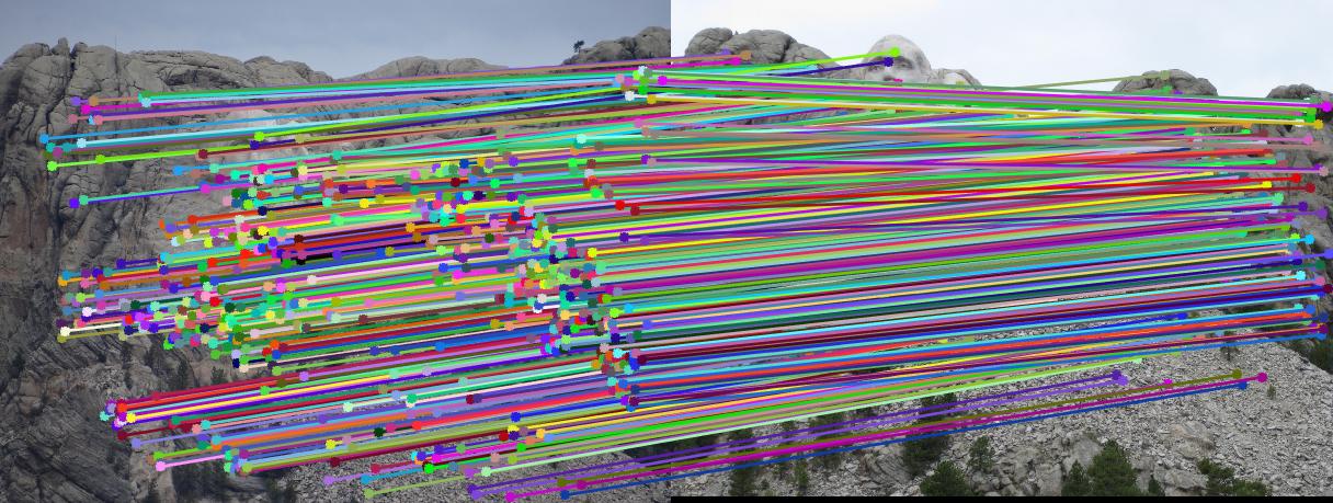
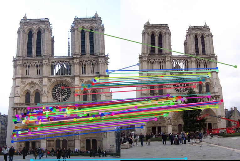
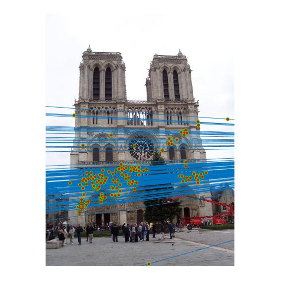
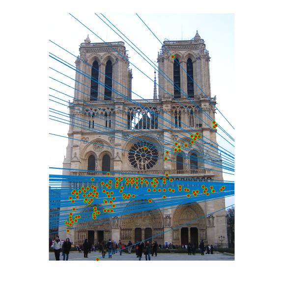
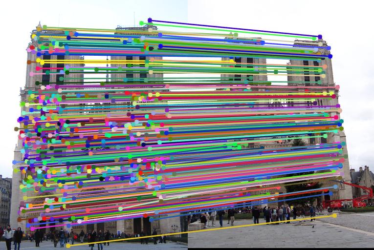
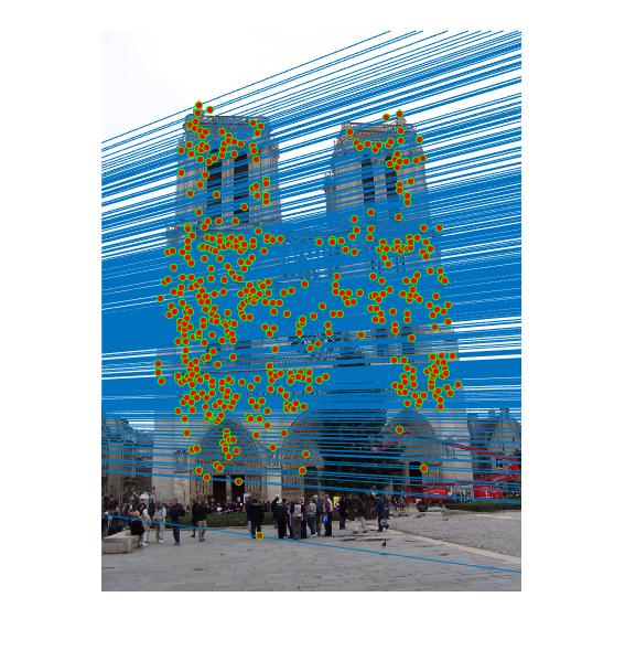
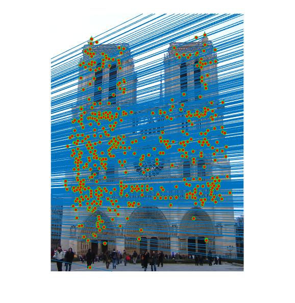
Before normalization the number of inliers detected were around 140 to 160 with threshold = 0.005. But by normalizing the data, the inliers increase more than triple. It lies in 600 to 700 with same threshold. We can even see the difference in the diagram. The faulty points also consideralbly reduce after normalizing the data.

Results in a table

Nortre Dam

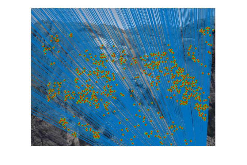
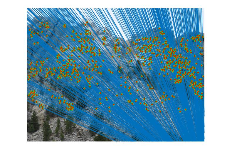
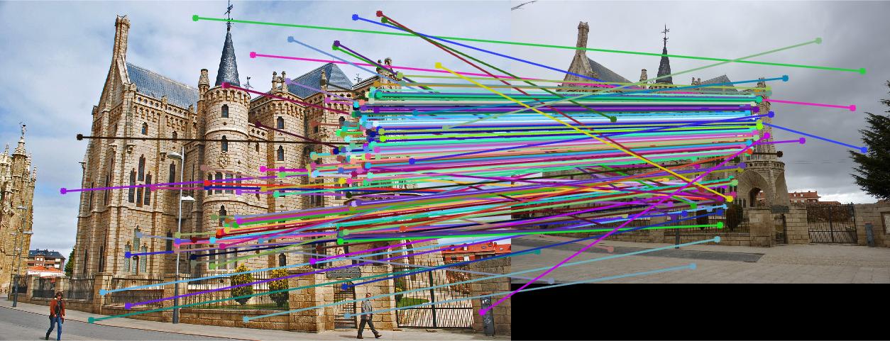
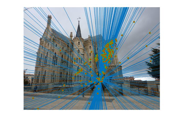
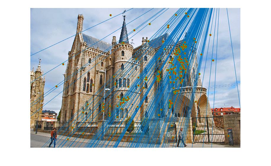
Episcopal Gaudi
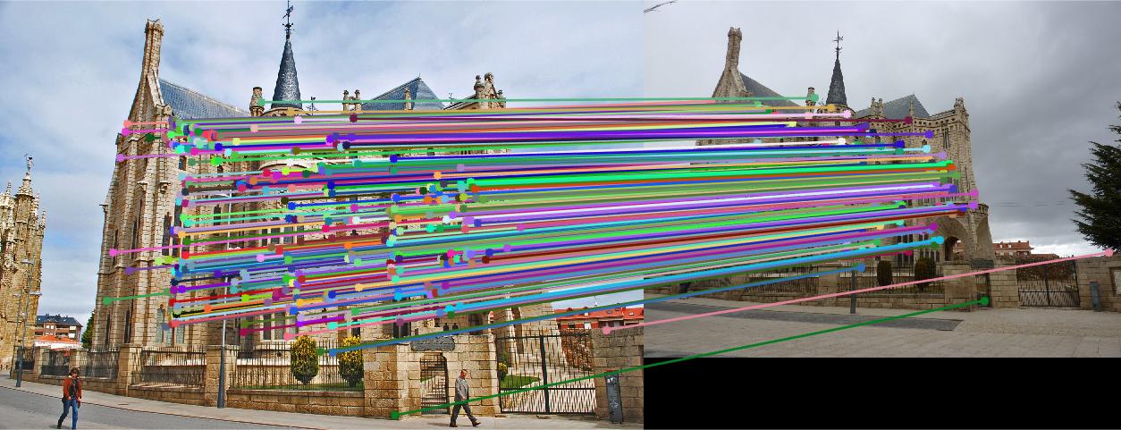
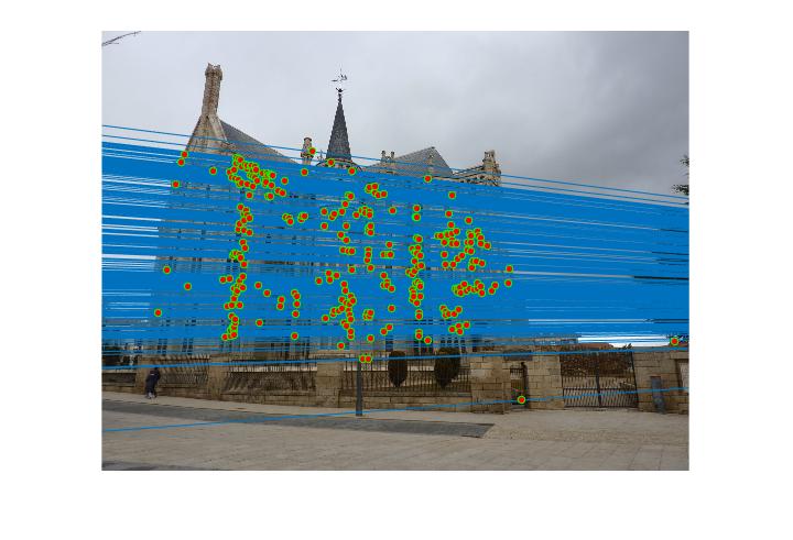
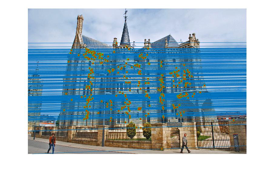