Computer Vision Project

For this project, I created some helper functions for parts 1, 2, and my attempt of the graduate credit. All of my helper methods begin with "setup_" followed by the matrix created by the function. To calculate the projection matrix, I called one of my helper functions to create the linear system for me, then I used the singular value decomposition method from lecture 13, slide 36 to solve for the system. My helper function is called "setup_nx12_homogeneous_matrix" and returns this matrix in the comments (X_i, Y_i, Z_i are from the 3D set of points, while u_i and v_i are from the 2D set of points, M is the projection matrix in vector form for which we wish to solve):

Loop through the 2n rows of points, if i is odd, append a row of the first form. If i is even, append a row of the second above form.

The projection matrix is:

[ [-0.4583 0.2943 0.0092 -0.0057]; [ 0.0508 0.0545 0.5411 0.0517]; [-0.1105 -0.1776 0.0479 -0.5968] ]

Also, my calculated residual is 0.0698 and the estimated location of camera is: [1.5115, 2.3430, -0.2825]

About the Fundamental Matrix and Graduate Credit:

The linear system I set up uses this formula from the slides: (f_11)uu' + (f_12)uv' + (f_13)u + (f_21)vu' + (f_22)vv' + (f_23)v + (f_31)u' + (f_32)v' + f_33 = 0. The sets of points and vectors are built into a matrix multipled by the vector [uu' uv' u vu' vv' v u' v' 1] by which we need to solve for the first 8 variables using the same trick I applied to part 1. I then estimated the fundamental matrix itself using lecture 13, slide 36 from class. The same code that appeared on that slide:

[U, S, V] = svd(Perms_of_pts);
F_matrix = V(:, end);
F_matrix = reshape(F_matrix, [3, 3])';

yielded the following matrix:

[ [-0.0000 0.0000 -0.0009]; [0.0000 0.0000 -0.0264]; [-0.0019 0.0172 0.9995] ]

As for the graduate credit, I chose to create a method known as "setup_transformation_matrix_for_normalization", where I calculated the mean coordinates for a list of points and the standard deviation from that. The standard deviation's magnitude is the reciprocal of the scale I used for my transformation matrix, but alas, it makes the epipolar lines disappear, so it is commented out in part 2. The code looks like this:

% "estimate the standard deviation after substracting the means"

standard_deviation_sq = 0;
for i=1:size(list_of_pts, 1)
    offset_u = list_of_pts(i, 1) - mean_coord_u;
    offset_v = list_of_pts(i, 2) - mean_coord_v;
    offset_sq_u = offset_u * offset_u;
    offset_sq_v = offset_v * offset_v;
    
    standard_deviation_sq = standard_deviation_sq + offset_sq_u + offset_sq_v;
end
% "Then the scale factor s would be the reciprocal of whatever estimate of
% the scale you are using"
scale = 1.0 / sqrt(standard_deviation_sq);

means_matrix = [1 0 (-1*mean_coord_u); 0 1 (-1*mean_coord_v); 0 0 1];
scale_matrix = [scale 0 0; 0 scale 0; 0 0 1];

T = scale_matrix * means_matrix;

When I estimated the fundamental matrix of my system, it was rank 1, and epipolar lines appeared through the image until I took the det(F) = 0 constraint into account. Once I took this constraint into account (see code below), the fundamental matrix stayed the same, but the epipolar lines disappeared! Similarly, applying the transformation matrices to normalize F merely zero-ed all but the the last entry of F, in which the epipolar lines disappeared completely. Thus, I have commented out that part of the code, which is below:

after applying noramlization:

[ [-0.0000 0.0000 -0.0000]; [ 0.0000 0.0000 -0.0000]; [-0.0000 0.0000 1.0034] ]

The code that made the epipolar lines disappear:

[uf,sf,vf] = svd(F_matrix);
sf(3, 3) = 0;
F_matrix = uf*sf*(vf)'; 
F_matrix = transpose(Tb) * F_matrix * Ta;

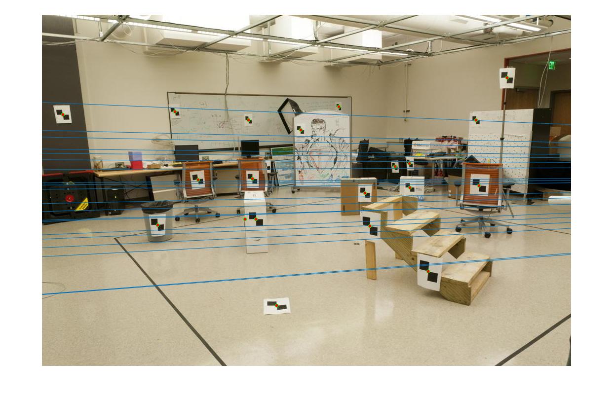
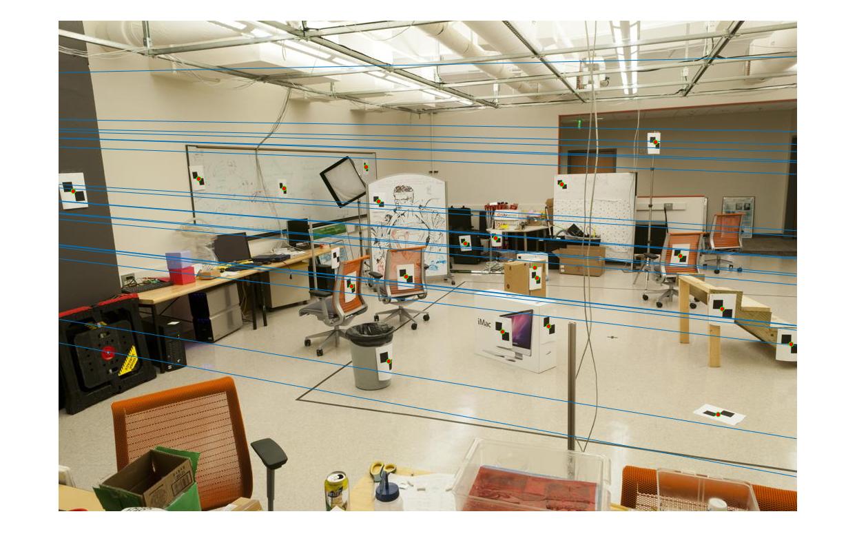
below are my epipolar lines for part 2:

Part 3:

I took the first 10 points from matches_a and matches_b and solved for the fundamental matrix. Ironically, the first line of the starter code's placeholder suited my method. I initialized a threshold for the distance metric between a pair of points using the fundamental matrix. The better the correspondence between the points, the closer to 0 this formula: [u' v' 1] * F * [u; v; 1] should be. Take the points with the smallest deviation, of which I found 31 for a threshold of 10,000.

Adding matches in the straightforward way using a loop:

if(abs(fundamental_value) < threshold)
            	inliers_a = [inliers_a; matches_a(i,:)];
                inliers_b = [inliers_b; matches_b(i,:)];
end

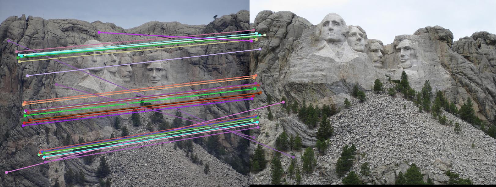
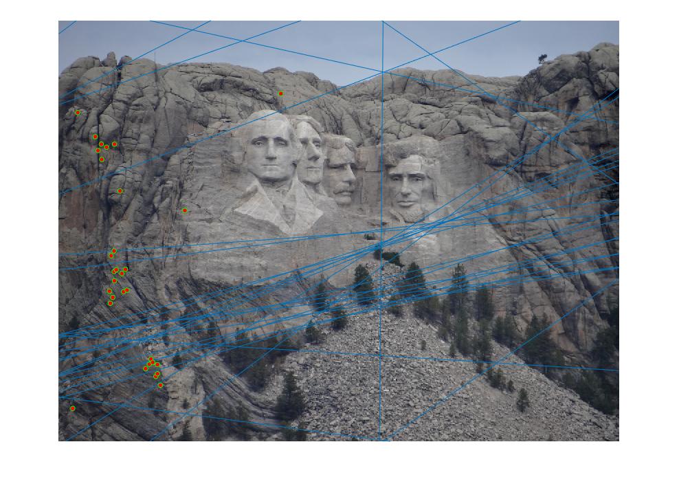
below are my epipolar lines and correspondence for part 3:

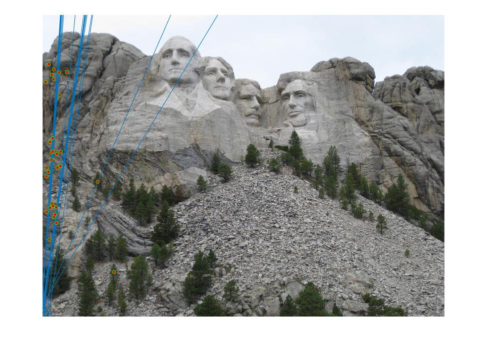
and correspondence between mount rushmore images for part 3:

Kristian Eberhardson

Project 3 / Camera Calibration and Fundamental Matrix Estimation with RANSAC