Project 3 / Camera Calibration and Fundamental Matrix Estimation with RANSAC
Camera Calibration.
The goal of this project is acheving high accuracy feature matching between pair of images by first estimating the camera projection matrix, which maps 3D world coordinates to image coordinates, as well as the fundamental matrix, which relates points in one scene to epipolar lines in another. Following this, the fundamental matrix estimation and RANSAC optimization are implemented, which are part of the feature point matching
- Estimation of Projection Matrix and Camera Centre
- Calculation of Fundamental Matrix
- Best Fundamental Matrix using RANSAC
Estimation of Projection Matrix and Camera Centre
The projection matrix is a linear transformation which aims to convert the real world 3D points to image 2D points. To estimate the projection matrix is to solve the M using linear algebra on the given point pairs. It also includes the effect of rotation and translation of the camera away from the origin
Example of code
[M , ~] = size(Points_3D);
A = zeros(M*2, 11);
A(1:2:end) = [Points_3D ones(M, 1) zeros(M, 4) -Points_2D(:,1).*Points_3D(:,1) -Points_2D(:,1).*Points_3D(:,2) -Points_2D(:,1).*Points_3D(:,3)];
A(2:2:end) = [zeros(M, 4) Points_3D ones(M, 1) -Points_2D(:,2).*Points_3D(:,1) -Points_2D(:,2).*Points_3D(:,2) -Points_2D(:,2).*Points_3D(:,3)];

B = reshape(Points_2D', M*2, 1);

 M = A \ B;
 M = [M ; 1];
 M = reshape(M, [], 3)';

% Calculating camera centre:

Q = M(:, 1:3);
m4 = M(:, 4);
Center = - inv(Q) * m4;
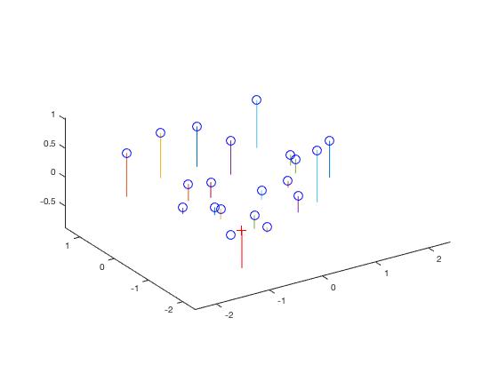
Results
The residue value obtained should be as small as possible and is found to be 0.0445 for the test images provided. The projection matrix obtained is shown below.
| M = | |||
| 0.7679 | -0.4938 | -0.0234 | 0.0067 |
| -0.0852 | -0.0915 | -0.9065 | -0.0878 |
| 0.1827 | 0.2988 | -0.0742 | 1.0000 |
The estimated location of camera is: <-1.5126, -2.3517, 0.2827>
Calculation of Fundamental Matrix
Like part one, part two is to estimate the fundamental matrix, which is a linear transformation between 2 images, both 2D points. Setting the last value to 1 for scaling helps in achieving consistency and can solve the system of equations for the 8 corresponding points. SVD is taken for this matrix to get matrices U, S and V. The last column of V is gives the fundamental matrix when reshaped to a 3 x 3 matrix. Then enforcing of the rank to be 2 is done.
Example of code
%example code

    % Perform normalization as mentioned in the assignment page

    %Calculating mean
    cuv_a = mean(Points_a);
    cuv_b = mean(Points_b);

    %Assigning the mean coordinates for transformation
    C_a = [1 0 -cuv_a(1); 0 1 -cuv_a(2); 0 0 1];
    C_b = [1 0 -cuv_b(1); 0 1 -cuv_b(2); 0 0 1];

    % recommended value of average magnitude
    std_est_scale = power(2, 0.5);

    % Computing scale s by estimating the standard deviation after substracting the means
    a1_std = std(Points_a(:,1) - cuv_a(1));
    a2_std = std(Points_a(:,2) - cuv_a(2));
    b1_std = std(Points_b(:,1) - cuv_b(1));
    b2_std = std(Points_b(:,2) - cuv_b(2));

    %std of both points
    std_a = a1_std + a2_std;
    std_b = b1_std + b2_std;

    %scale s of both points
    scale_a = std_est_scale / std_a;
    scale_b = std_est_scale / std_b;

    % Matrix for scaling (transformation)
    S_a = [scale_a 0 0; 0 scale_a 0; 0 0 1];
    S_b = [scale_b 0 0; 0 scale_b 0; 0 0 1];

    % Transforming the matrix
    Transform_A = S_a * C_a;
    Transform_B = S_b * C_b;
    Points_a(:, 3) = 1;
    Points_b(:, 3) = 1;

    % normalize the points
    Temp_a = Transform_A * Points_a';
    Points_a = Temp_a';
    Temp_b = Transform_B * Points_b';
    Points_b = Temp_b';

    [num_rows, ~] = size(Points_a);
    W = ones(num_rows, 8);
    for each = 1 : num_rows
        W(each, :) = [Points_a(each, 1) * Points_b(each, 1), Points_a(each, 2) * Points_b(each, 1), Points_b(each, 1), Points_a(each, 1) * Points_b(each, 2), Points_a(each, 2) * Points_b(each, 2), Points_b(each, 2), Points_a(each, 1), Points_a(each, 2)];
    end

    % Extracting the fundamental matrix and reshaping
    F = W \ -ones(num_rows,1);
    F(9) = 1;
    F_matrix = reshape(F, [3, 3])';

    % Enforce constraint of rank = 2
    [U, S, V] = svd(F_matrix);
    F_matrix = U * diag([S(1,1) S(2,2) 0]) * V';


    % normalize the fundamental matrix - allow it to operate o original
    % pixel coordinates
    F_matrix = Transform_B' * F_matrix * Transform_A;
We can visualize the epipolar lines as follows:
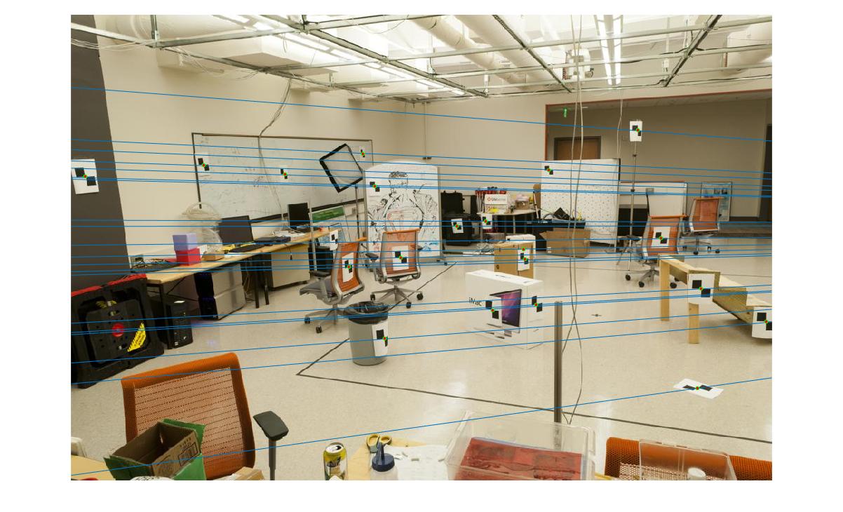
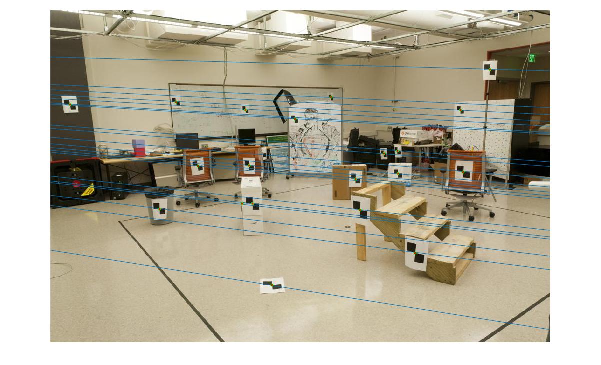
|
Fundamental Matrix Using RANSAC
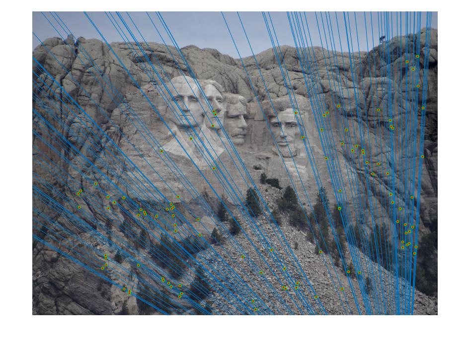
The final part is to find the best fundamental matrix using the RANSAC based on the matched points given by SIFT. The SIFT is run to extract matching features. Randomly 8 points are sampled to generate the fundamental matrix. The entire feature set is now multiplied by the fundamental matrix and the number of inliers calculated. This process is iterated many number of times and various tresholds are set and compared for best results. Any points with the distance from the expected value drived from fundamentall matrix are considered as inliers, and others are outliers. The best fundamental matrix is selected as the one having maximum number of inlier points.
Example of code
%example code
inliner_max_count=0;
    threshold_val = 0.05;
    maxloop = 3000;
    counter = 0;
    rows = size(matches_a,1);

    while counter < maxloop

        %compute F_matrix with random points sampled from A and B
        random_pts=randsample(rows,8);
        sample_a = matches_a(random_pts, :);
        sample_b = matches_b(random_pts, :);
        F_matrix=estimate_fundamental_matrix(sample_a, sample_b);

        % Assign inliner to be 0 and increment for each "inliner" found
        % distances should be less than the treshold value
        inlier_count=0;
        for i=1:rows
            B = [matches_b(i, :) 1];
            A = [matches_a(i, :) 1];
            distance= B*F_matrix*A';
            if abs(distance)< threshold_val
                inlier_count=inlier_count+1;
            end
        end

        if(inlier_count>inliner_max_count)
                inliner_max_count=inlier_count;
                Best_Fmatrix=F_matrix;
        end

        counter = counter + 1;
    end

    final_points=zeros(rows, 1);

    for count=1:rows
        B = [matches_b(count, :) 1] ;
        A = [matches_a(count, :) 1]';
        final_points(count)=abs(B*Best_Fmatrix*A);
    end

    [~, inlier]=sort(final_points);
    inliers_a=matches_a(inlier(1:inliner_max_count),:);
    inliers_b=matches_b(inlier(1:inliner_max_count),:);
The above code shows that normalization is done. The results drastically improve after normalization. I use the method given in the question to consider root_2 and find the std between the points and the mean and adjust the points based on the mean and calculate the standard deviation ratio.
Mount Rushmore
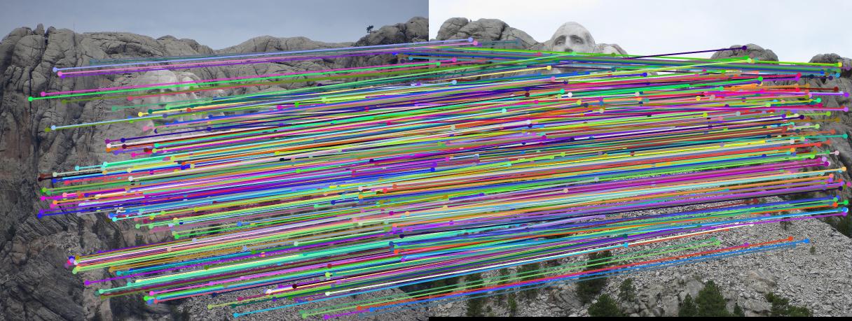
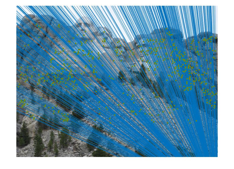
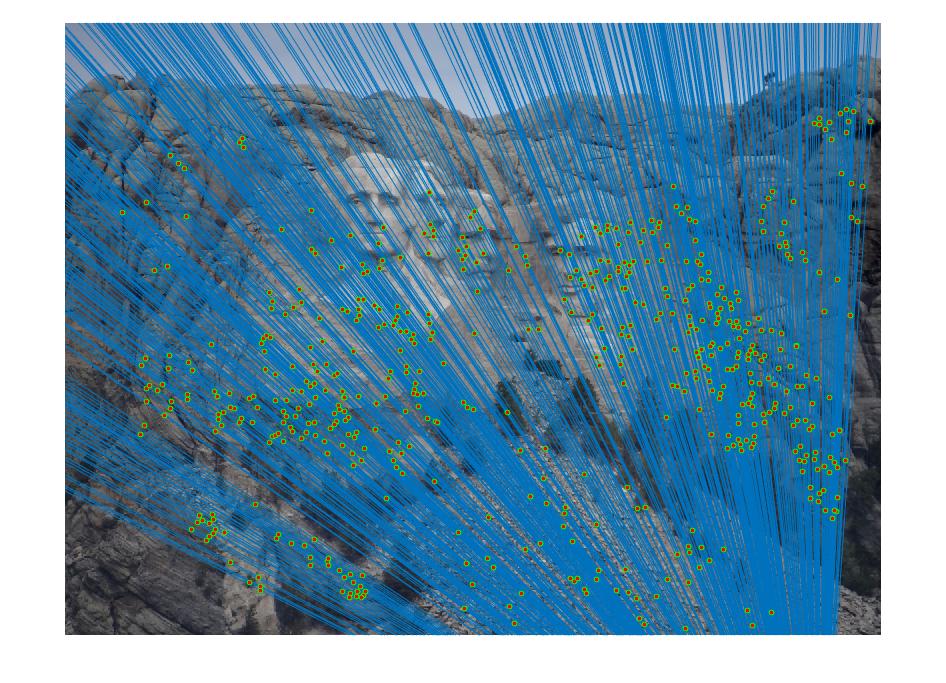
|
Mount Rushmore with treshold as 0.10
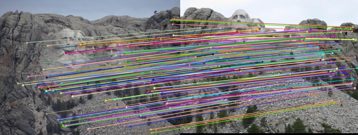
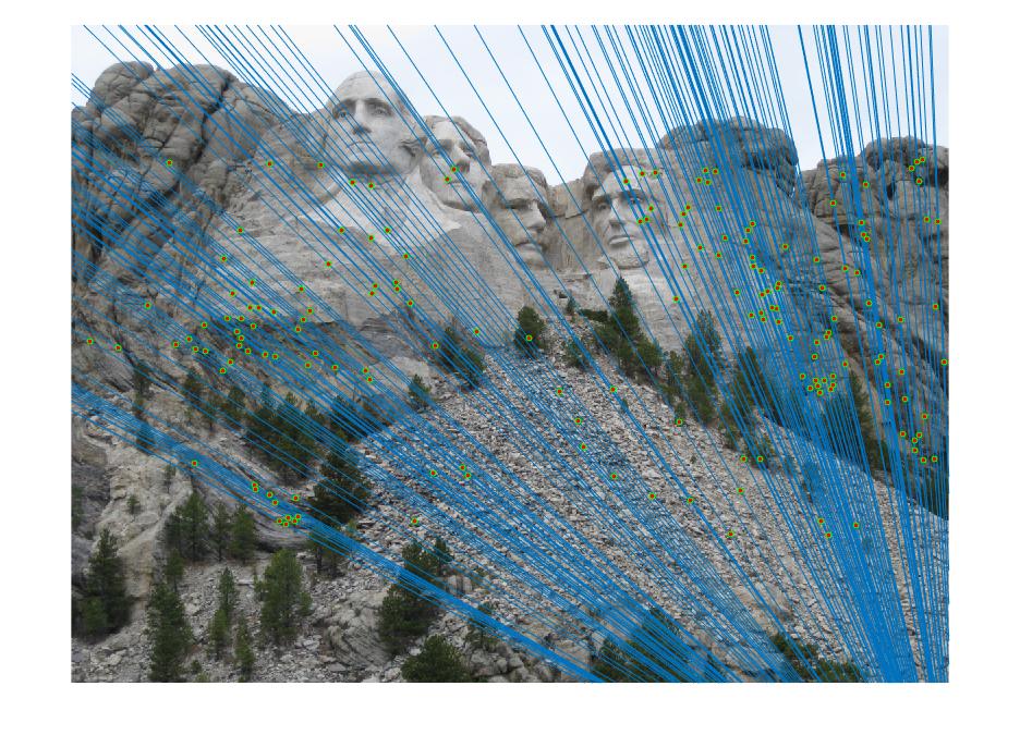
|
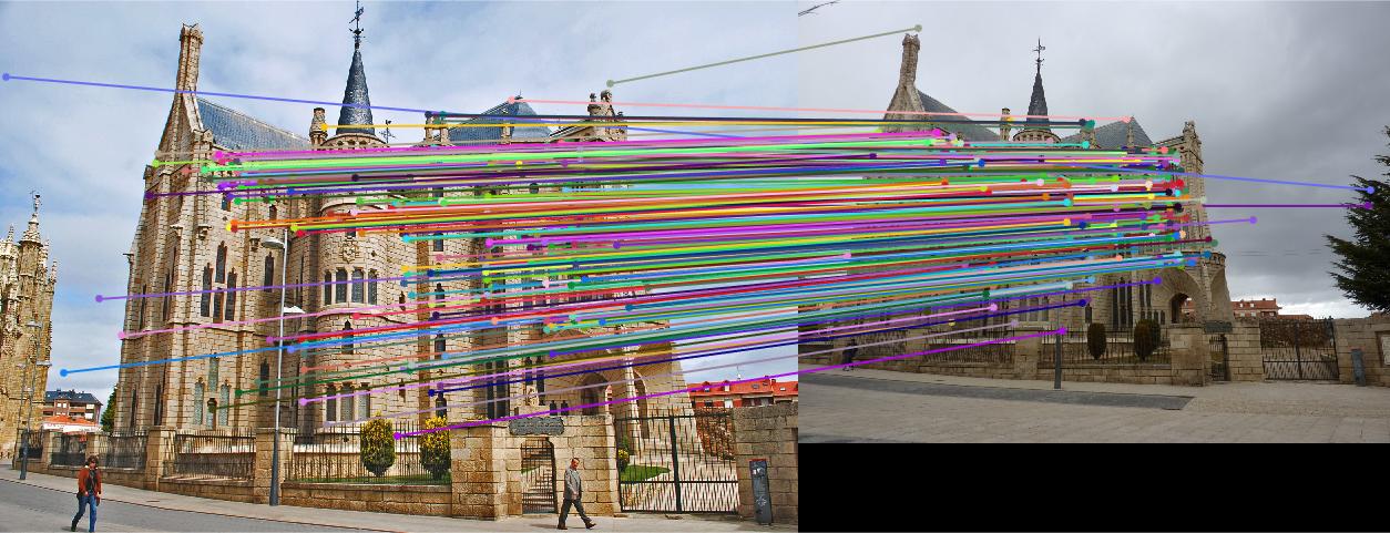
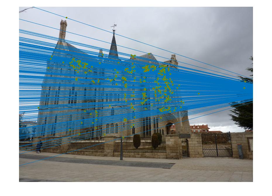
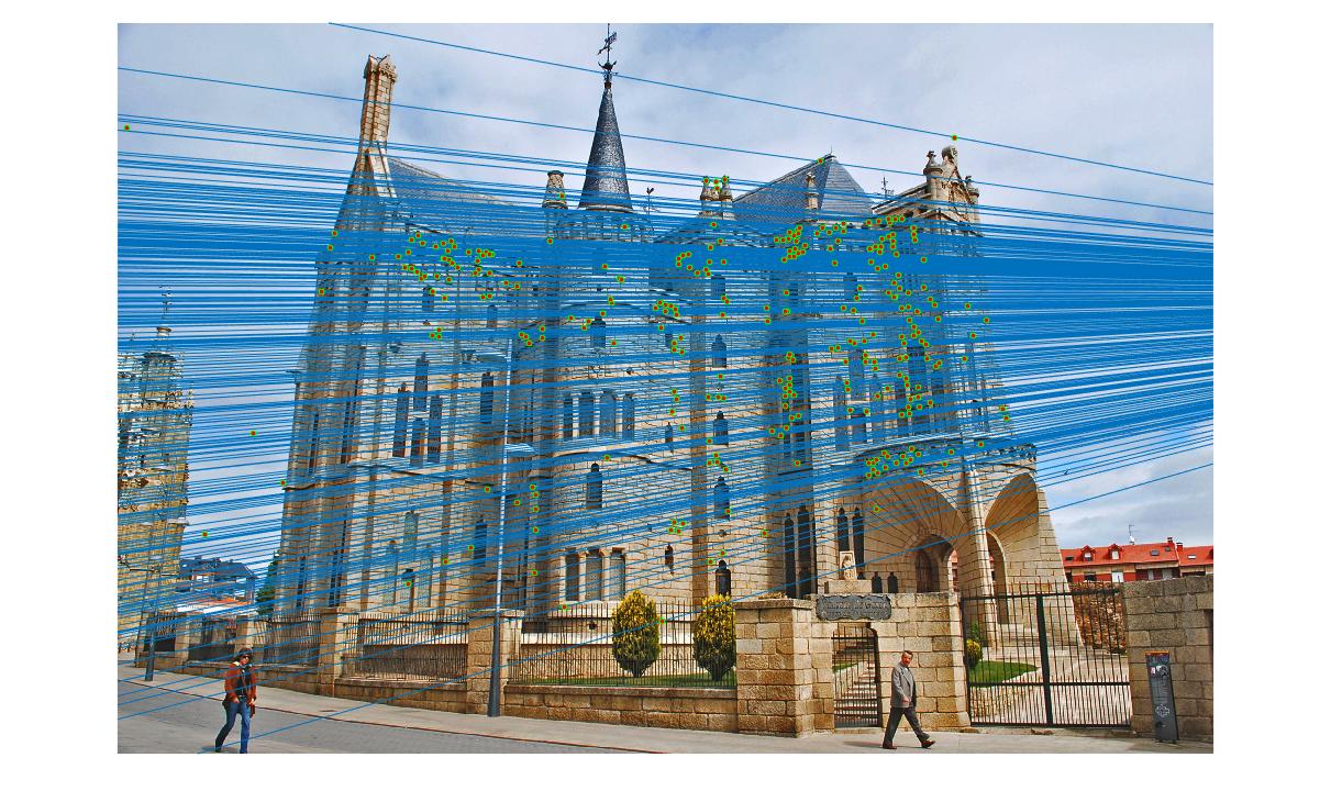
Episcopalian Gaudi
|
Notre Dame
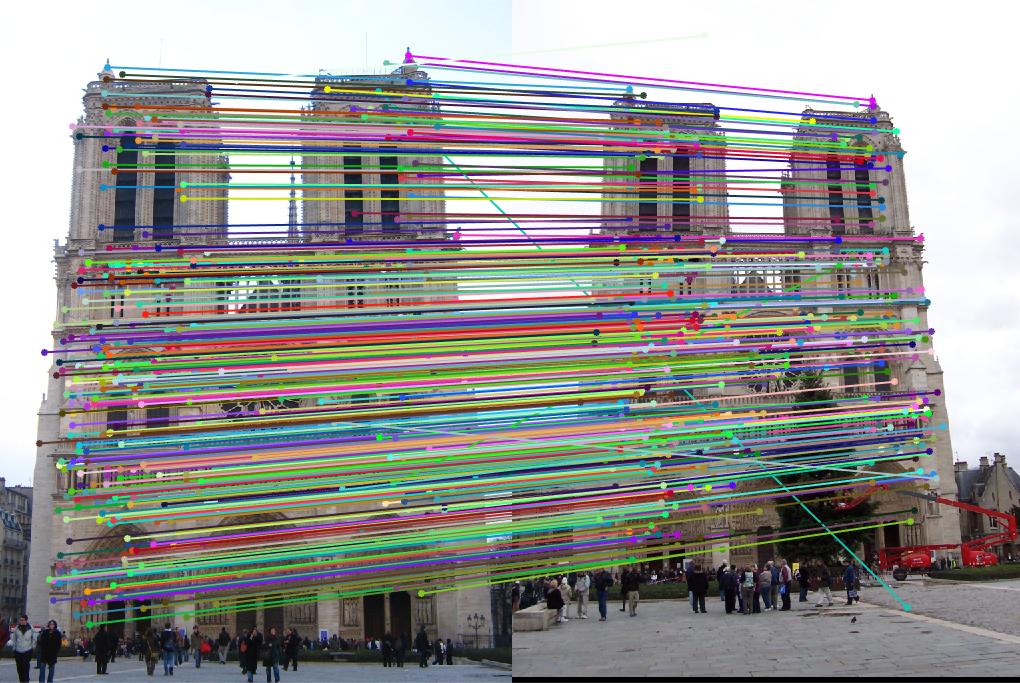
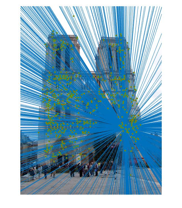
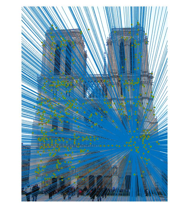
|
As seen in the above results, varying the treshold value also plays a role while finding the number of inliers when RANSAC is run. Lowering the value of treshold means more strict conditions and hence lesser number of inliers are obtained