Project 3 / Camera Calibration and Fundamental Matrix Estimation with RANSAC
Understanding depth in a 2-D image is a lot harder than it looks (yay for puns). Afterall, going from 3-D to 2-D images is by definition dimensionality reduction, which means that at least some information will be lost. In this project, we'll explore various approaches to uncovering and exploiting the relationship between 2-D and 3-D points in images.
Camera Projection Matrix
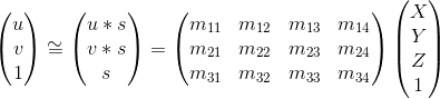
We can view the process of going from 3-D to 2-D points as a linear transformation. Luckily for us, given enough points, we can solve for said linear transformation and be able to project any 3-D point into the 2-D plane. The general form of the transformation is shown below. If we do some nice and rearranging, we'll get the equation directly below the projection formula.
Projecting from 3-D to 2-D.

Simplified form of the projection above
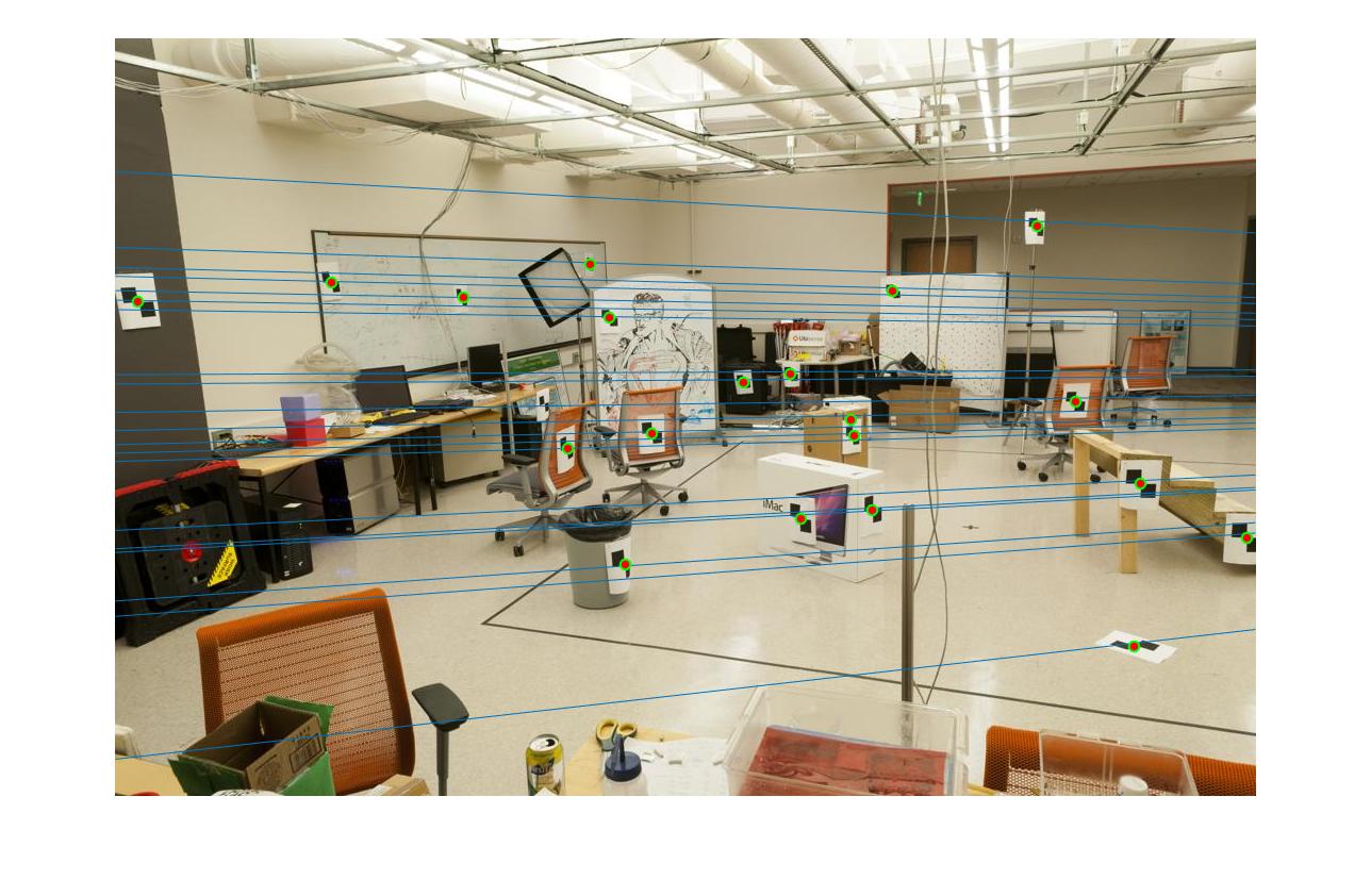
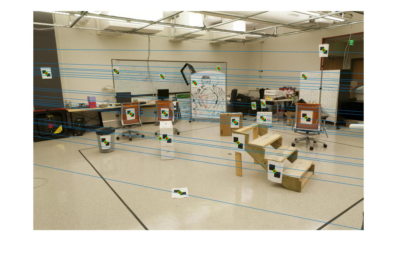
What makes the equation above nice is that given at least 8 points, we can then solve directly for each value in the transformation matrix. The only problem is that the trivial solution (i.e. all zeros) is always a solution. To get around this, I constrained the last element at index 3,4 to be 1. I then used least squares to find the remaining coefficients. Given a groundtruth set of points in 3D space and their corresponding 2D, this approach does a good job of estimating the projection matrix. The image below shows the result of projecting 3D points onto the 2D space. While this is a slight amount of difference, it clearly captures the main information. My residual was 0.0445
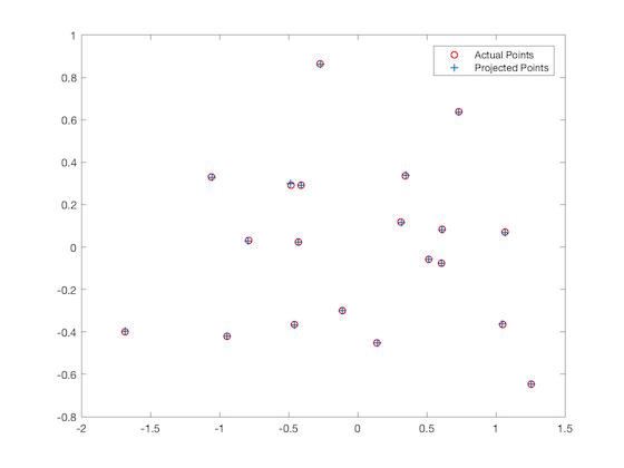
Results of camera projection
One additional insight we can tease out of this transformation matrix is the camera center. Using some math given in the lecture slides, we can get a nice result for the camera center as shown below.
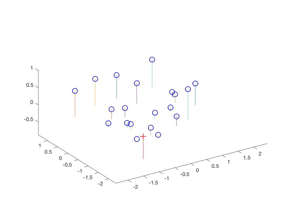
Results of camera projection
Fundamental Matrix Estimation
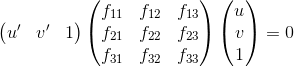
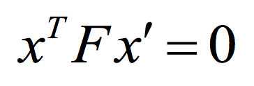
Given two scenes from different perspectives, can we intelligently map points from one to another? The answer is yes, by means of the fundamental matrix. The fundamental matrix is defined below for two points corresponding points. Similarly to above, this can be reduced to a nice homogenous equation, as shown below.
Fundamental Matrix

Alternative form of the Fundamental Matrix
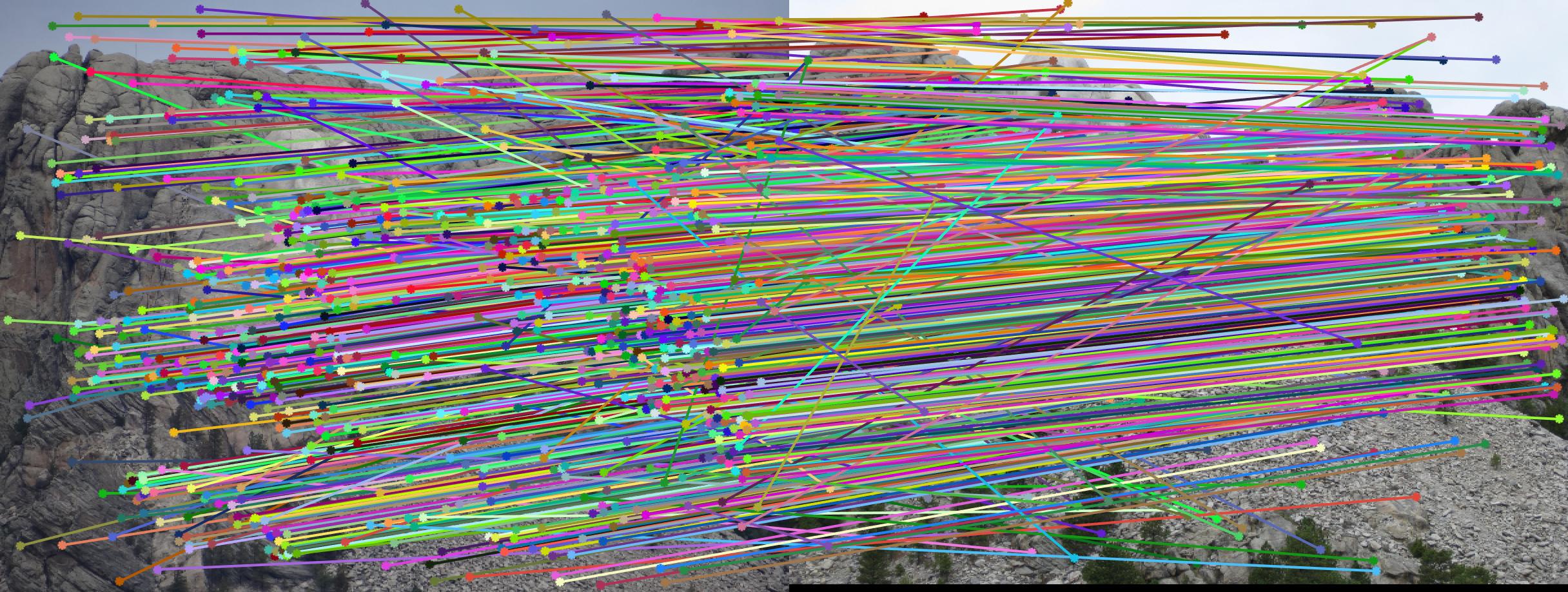
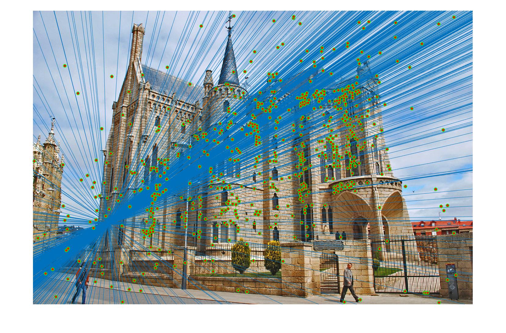
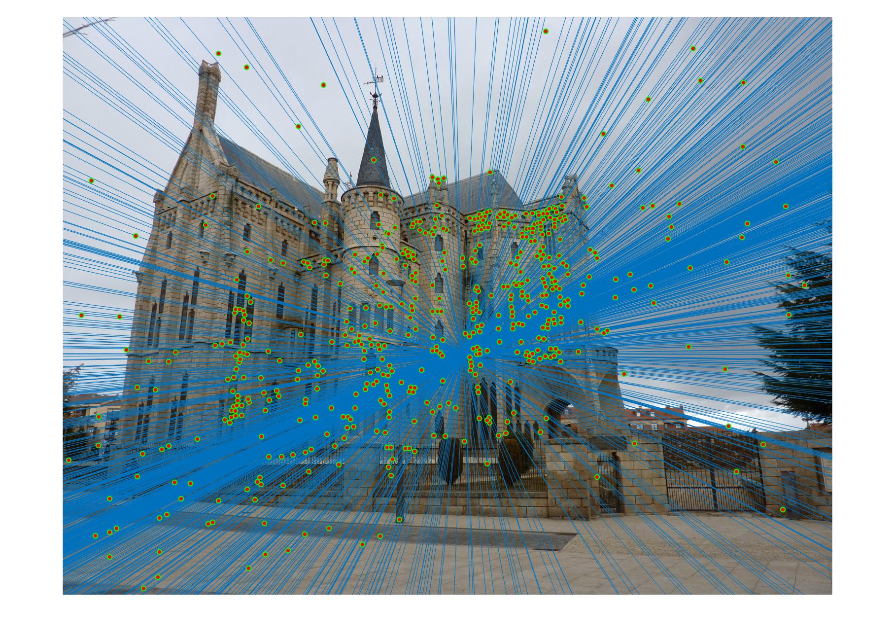
Given enough corresponding points (at least 8, since there are 8 unknowns), the values of the fundamental matrix estimation can be estimated using least squares, just like in part one. The only difference is that the estimate of F is full rank, while the fundamental matrix is rank 2. I dealt with this according to the instructions of the project. Once the fundamental matrix has been calculated, the epipolar lines can be drawn. A good estimate should have the lines cross through the corresponding points in the other image. Here are my epipolar results given below. Though it's not perfect, the lines clearly do a good job of capturing the points.
Epipolar Lines of Corresponding Images
|
Fundamental Matrix Estimation with RANSAC
The fundamental matrix that generated the epipolar lines above was calculated using ground truth correspondences. This leads to the best results, as there is no noise to disorient the matrix. In most situations, we won't be lucky. So we have to adopt our stategy to still get an accurate fundamental matrix given a large number of correspondonets, some of which may be wrong. To do this, we'll use RANSAC. The idea is simple. Sample a few correspondences (at least 8, I sampled 13) and estimate the fundamental matrix. Then count the number of inliers. Do this a certain number of times (I chose 1000 for this), and choose the matrix which has the most number of inliers. To find an inlier, we use the following fact.
Characteristic of the Fundamental Matrix
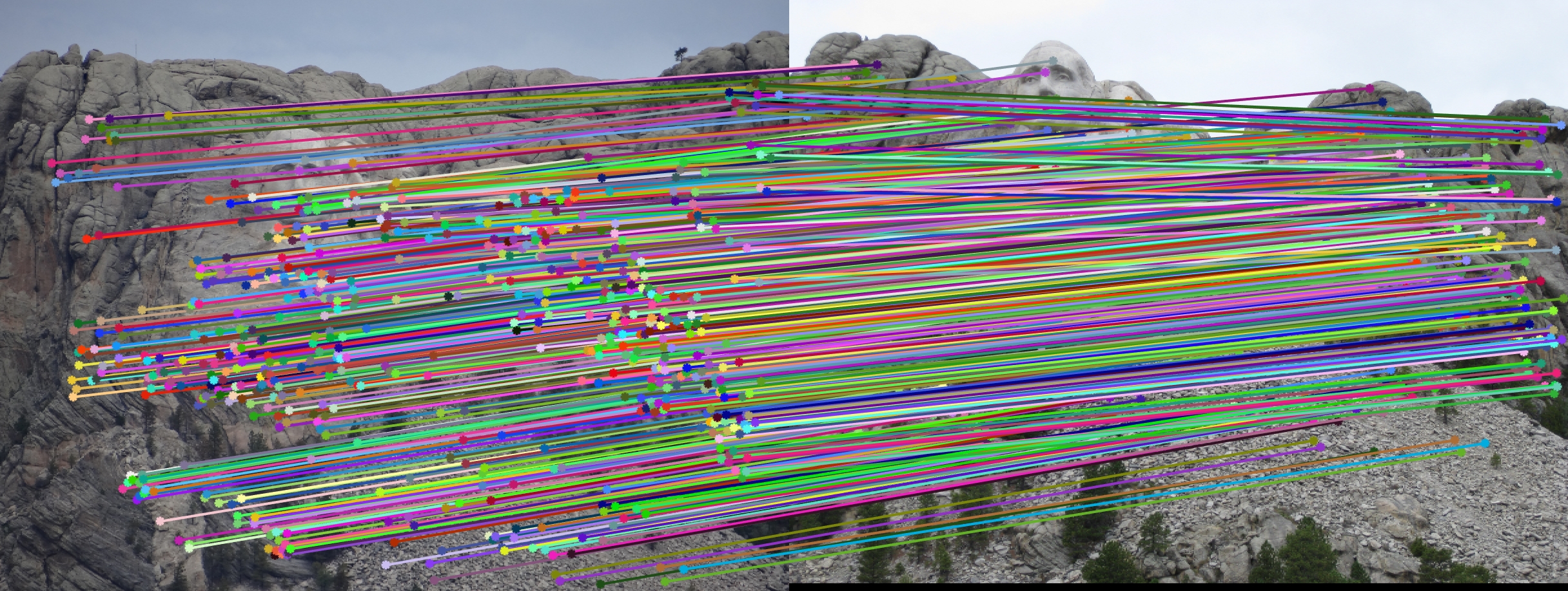
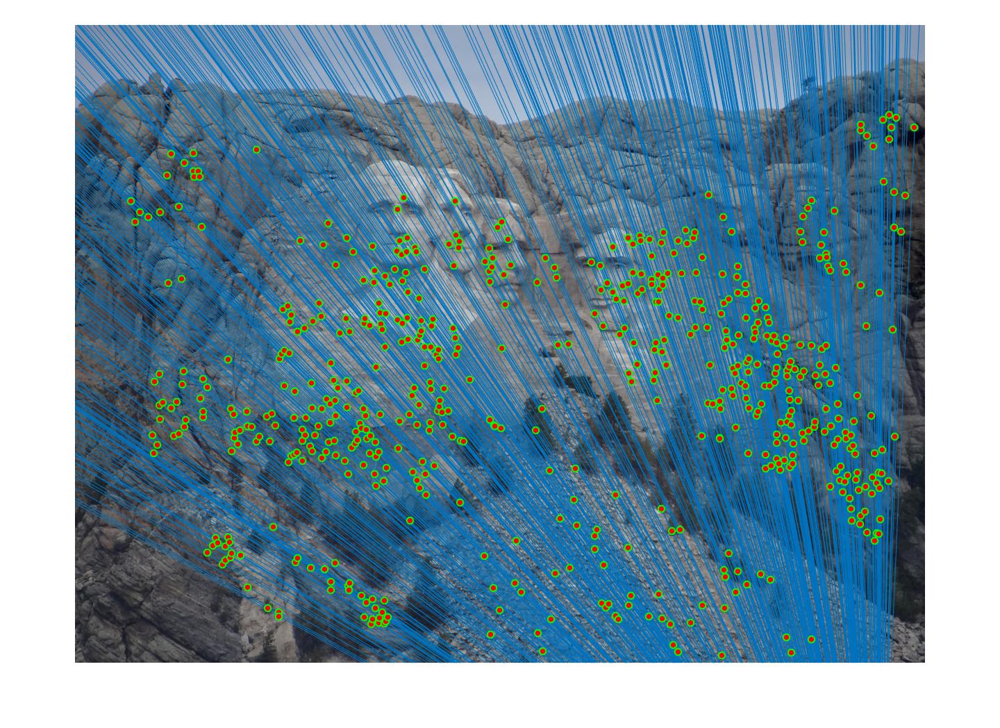
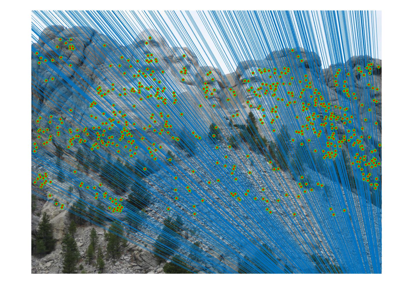
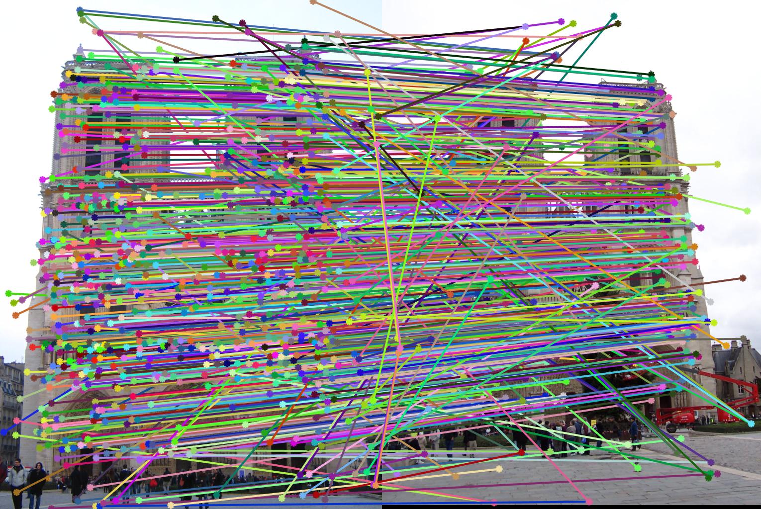
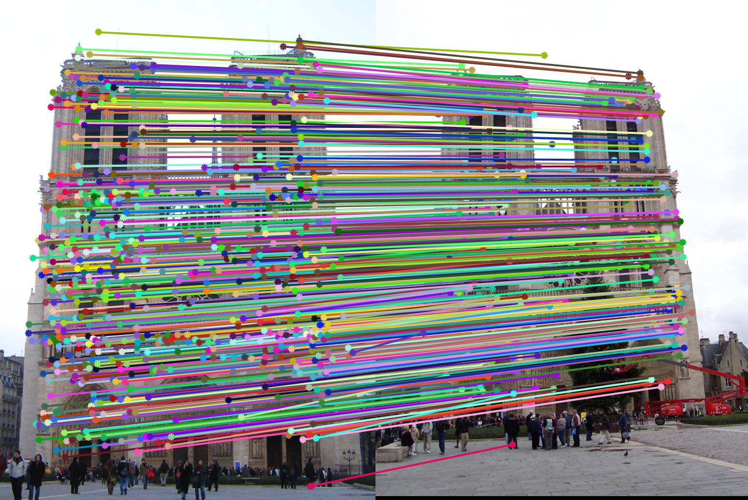
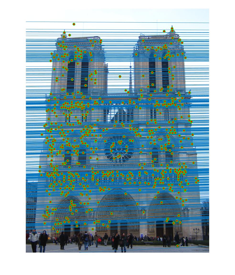
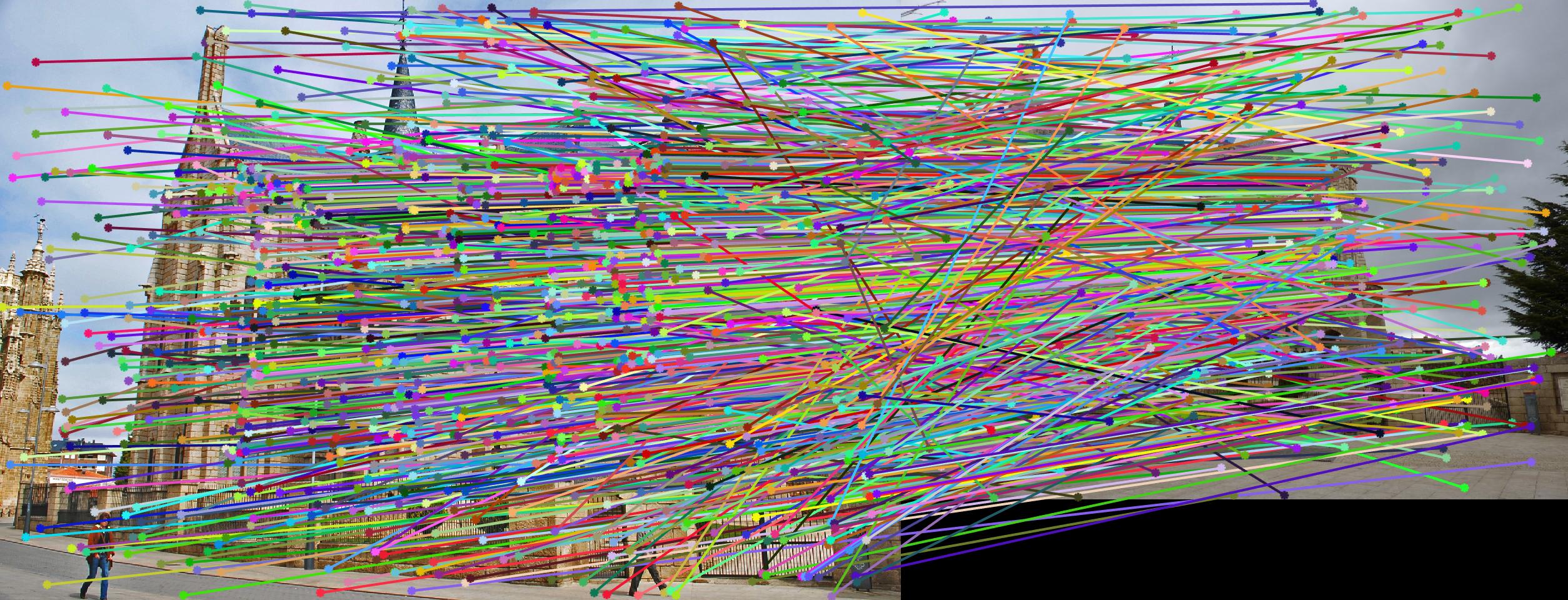
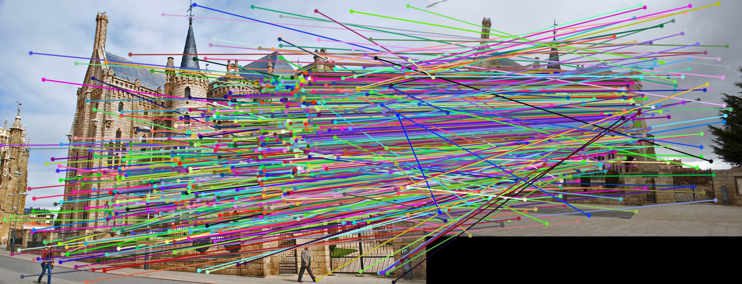
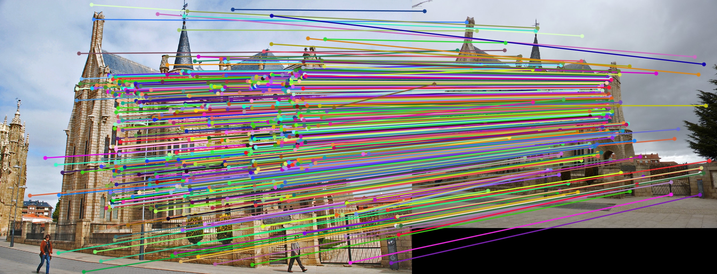
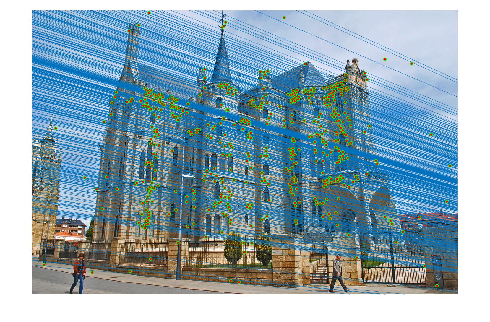
If the value is less than 0.05 for a correspondence when plugged into the equation above, I consider the correspondence an inlier. Once the fundamental matrix has been estimated, it can be used to discard incorrect SIFT features by throwing out points if they don't lie on the corresponding epipolar line. This approach does a good job for the easy images, but no so much for the Gaudi pair, as we can see below.
SIFT Feature Removal with No Normalization (Before and After, with epipolar lines underneath)
|
|
|
|
|
|
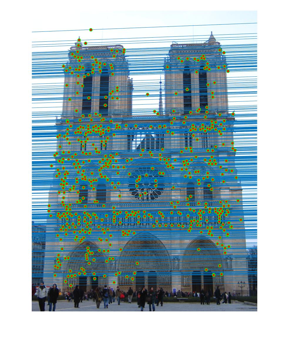
Luckily, we can improve the results dramatically with a small fix. The values used to calculate the f matrix can vary dramatically, leading to poor numerical stability. Thus, some sort of normalization scheme will lead to improved performance. To do this, I find the mean of the x and y coordinates of the correspondences used to estimate the fundamental matrix. I then subtract these means from each corresponce to zero center them. I then take the standard deviation of the resulting points and divide them by this number. This leads to much better results compared to the non-normalized approach.
SIFT Feature Removal with Normalization (Original on top, no normalization on left, normalization on right)
|
|
|
|