Project 3 / Camera Calibration and Fundamental Matrix Estimation with RANSAC
This project uses RANSAC and epipolar geometry between two images to match features between two images. The first part of the project calculates the projection matrix between a set of 2D and 3D points. This is used to find the camera center. The second and third parts attempt to estimate the fundamental matrix, which provides an epipolar relationship between points in two images. The best fundamental matrix is found using RANSAC, and the best-matching features are plotted.
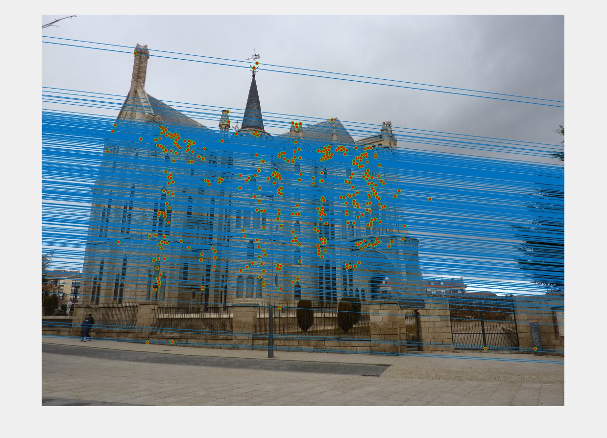
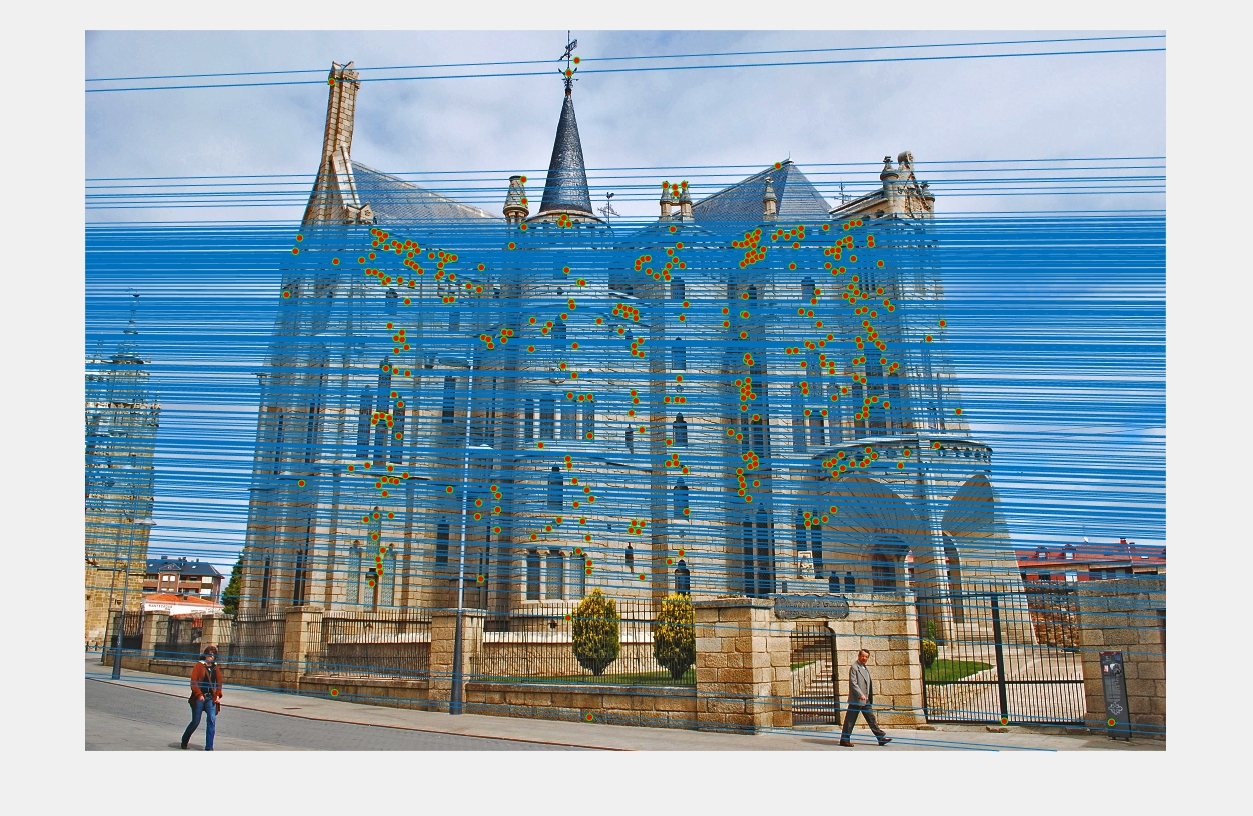
Epipolar lines on the Gaudi Episcopal Palace images
Part I: Camera Projection Matrix
The projection matrix is computed by using a least-squares regression between the set of 2D projected points and 3D real-world points. The projection matrix maps the 3D points to the 2D image plane. The code below explains how the regression was calculated.Using the computed fundamental matrix, the camera center was calculated to be
<-1.5126, -2.3517, 0.2827>.
% Construct the A and b matricies
for p=1:size(Points_2D, 1)
		...
    A(2*p - 1, :) = [X Y Z 1 0 0 0 0 -u*X -u*Y -u*Z ];
    A(2*p, :) = [0 0 0 0 X Y Z 1 -v*X -v*Y -v*Z ];

    b(2*p -1) = u;
    b(2*p) = v;
end

% Solve for values and normalize
M = A\b;
M = [M; 1];
M = reshape(M, [], 3)';
M = M/norm(M);
Part II: Fundamental Matrix Estimation
This part of the project attempts to find the fundamental matrix, a relationship between a point in one stero image to an epipolar line in the other. To estimate the fundamental matrix, a least-squares regression is used.
Extra Credit: Normalizing
I did the extra to normalize the points when calculating the fundamental matrix. For each image, I centered the points around the mean. I then found the scale for each such that the mean-squared distance was 1. This information was used to create the transformation matrices.
% Find means
mean_a = [mean(Points_a(:, 1)) mean(Points_a(:, 2))];
mean_b = [mean(Points_b(:, 1)) mean(Points_b(:, 2))];

% Center points around the means
Centered_a(:, 1) = Points_a(:, 1) - mean_a(1);
Centered_a(:, 2) = Points_a(:, 2) - mean_a(2);
Centered_b(:, 1) = Points_b(:, 1) - mean_b(1);
Centered_b(:, 2) = Points_b(:, 2) - mean_b(2);

% Get the mean squared error
err_a = 0;
err_b = 0;
for i=1:size(Centered_a, 1)
    err_a = err_a + (Centered_a(i, 1)^2 + Centered_a(i, 2)^2);
    err_b = err_b + (Centered_b(i, 1)^2 + Centered_b(i, 2)^2);
end

% Calculate scales such that the average squared distances are 1
s_a = sqrt(size(Centered_a, 1) / err_a);
s_b = sqrt(size(Centered_b, 1) / err_b);

% Create T matrices
T_a = [s_a 0    -s_a*mean_a(1); ...
       0   s_a  -s_a*mean_a(2); ...
       0   0     1];
T_b = [s_b 0    -s_b*mean_b(1); ...
       0   s_a  -s_b*mean_b(2); ...
       0   0     1];
After normalizing, the points must be multiplied by the transformation matricies to create the matrix A. The SVD is taken of A, to get F from the Value matrix. F is then denormalized, and the smallest singular value is removed so that the solution is of rank 2.
% Populate A matrix
for p=1:size(Points_a, 1)

    % Transform the original coordinates
    Trans_a = T_a*[Points_a(p, :) 1]';
    Trans_b = T_b*[Points_b(p, :) 1]';
    Ua = Trans_a(1);
    Va = Trans_a(2);
    Ub = Trans_b(1);
    Vb = Trans_b(2);

    A(p,:) = [Ua*Ub Va*Ub Ub Ua*Vb Va*Vb Vb Ua Va 1];
end

% Do SVD to get F
[U, S, V] = svd(A);
f = V(:, end);
F_matrix = reshape(f, [], 3)';

% Get F by denormalizing
F_matrix = T_b' * F_matrix * T_a;

% Remove the smallest singular value
[U, S, V] = svd(F_matrix);
S(3,3) = 0;
F_matrix = U*S*V';
The addition of the normalization did not appear to produce any more accurate results. It did increase computation time slightly, and the accuracy of point matches did not appear to increase with any statistical significance.
Part III: RANSAC
In this part of the project, RANSAC is used to find the best fundamental matrix solution that maps the epipolar lines between the two stero images. RANSAC performs the following steps:
- Randomly select the minimum number of point pairs to fit the model. In this case, 8
- Fit a model (the fundamental matrix) to the selected points. This was done using least-squares
- Evaluate the model based on the number of inliers. To classify an inlier, I used the distance from the feature point in image B to the epipolar line formed from
F*x, where x is the feature point in image A. - Select the fundamental matrix with the most inliers
    F = estimate_fundamental_matrix(samples_a, samples_b);
    a_tmp = [];
    b_tmp = [];
    for p=1:size(matches_a, 1)
        x = [matches_a(p, :) 1]';
        line_a = F*x;
        d = abs(line_a(1)*matches_b(p, 1) + line_a(2)*matches_b(p,2) + line_a(3))...
            / sqrt(line_a(1)^2 + line_a(2)^2);
        if d < 1
            a_tmp = [a_tmp; matches_a(p, :)];
            b_tmp = [b_tmp; matches_b(p, :)];
        end
    end

    if size(a_tmp, 1) > size(inliers_a,1)
        inliers_a = a_tmp;
        inliers_b = b_tmp;
        Best_Fmatrix = F;
    end
Results
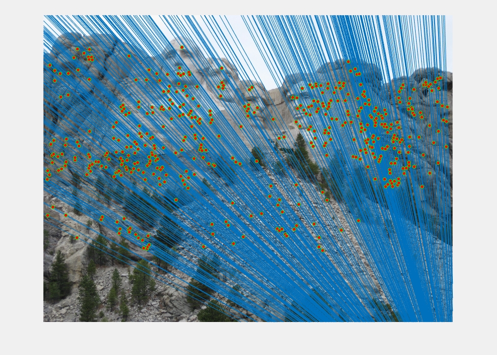
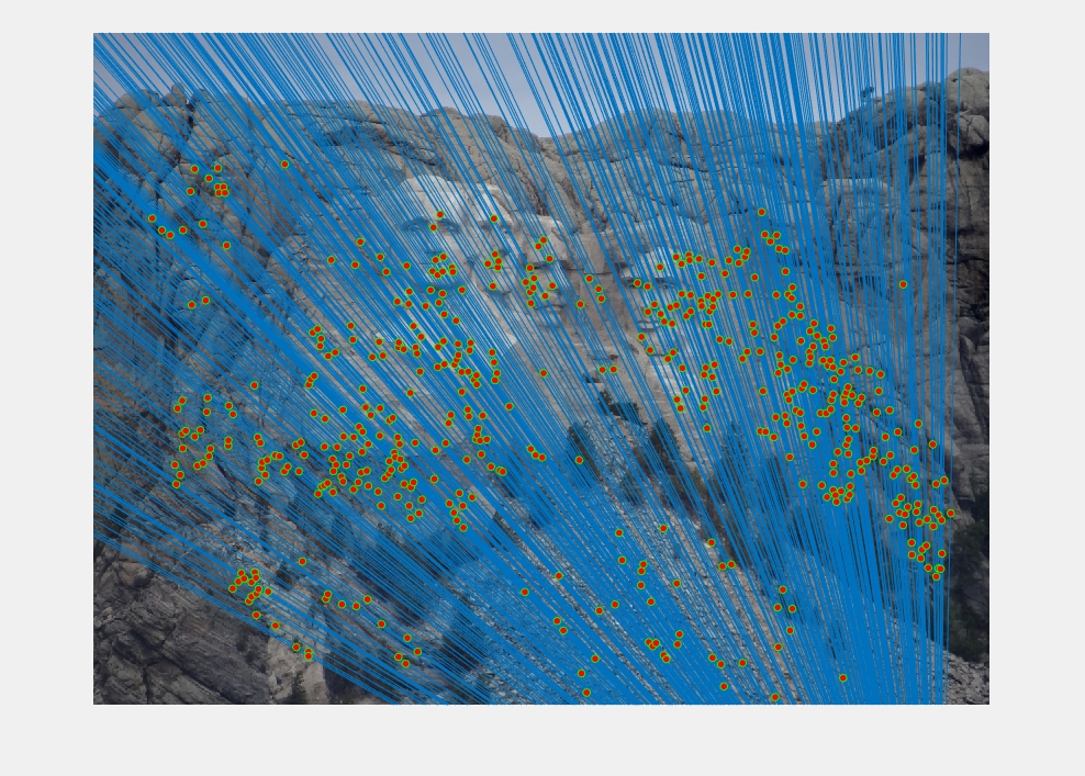

Epipolar lines and matches on the Mount Rushmore images. The epipolar lines are near vertical because of the downward translation of the images.
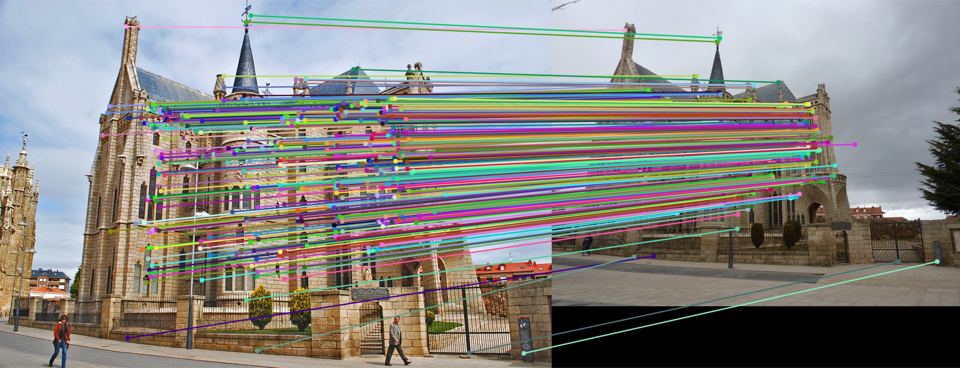
Epipolar lines and matchs on Gaudi Episcopal Palace. Excellent matches!
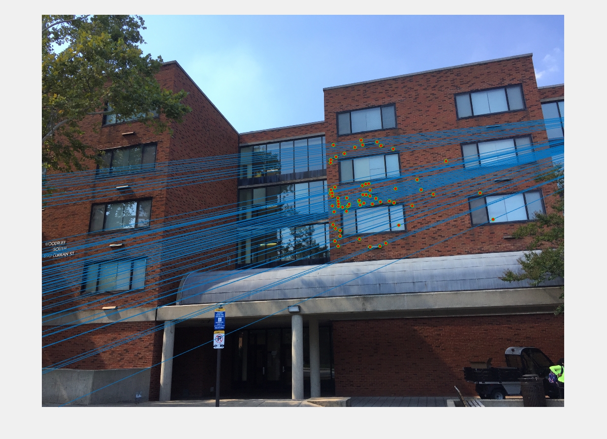
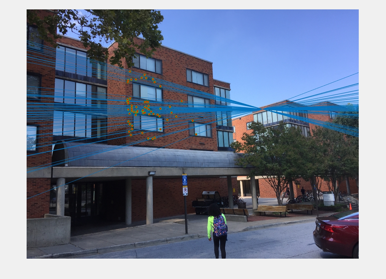
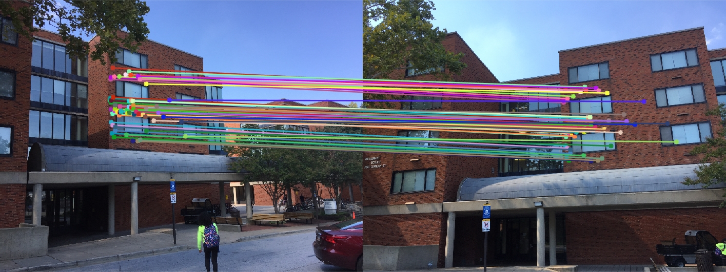
Epipolar lines and matchs on Woodruff dorm. The convergence of the lines at the epipole in the second image implies that the optical center (camera) of the first image is in the field-of-view of the second. From looking at the images, it is possible that is the case.