Project 3: Camera Calibration and Fundamental Matrix Estimation with RANSAC
Intro
This project had 3 parts. In the first part, I wrote code to find the camera projection matrix which converts 3D coordinates to 2D coordinates on the image. In part 2, I implemented a function to extimate the fundamental matrix given corresponding point locations in two images. In part 3, I used RANSAC to find a good fundamental matrix from SIFT feature matches.
Part I: Camera Projection Matrix
The projection matrix from world to image coordinates can be calculated with a system of equations which translates to an Ax=b matrix problem. My construction of the A and b matrices looks like this in Matlab:
a = [];
b = [];
for row = 1:size(Points_3D, 1)
    x = Points_3D(row, 1);
    y = Points_3D(row, 2);
    z = Points_3D(row, 3);

    u = Points_2D(row, 1);
    v = Points_2D(row, 2);

    row1 = [x y z 1 0 0 0 0 -u*x -u*y -u*z];
    row2 = [0 0 0 0 x y z 1 -v*x -v*y -v*z];
    a = [a;row1;row2];

    b = [b;u;v];
end
The calculation of x (the vector form of M, the projection matrix) looks like this:
x = a\b;
x = [x;1];
M = reshape(x, [4, 3])' ./ (.7679 / -0.4583); % (.7679 / -0.4583) does scaling
Next, I calculated the camera center using the equation C = -Q^(-1)m_4, given in the assignment. The code for that looks like this:
q = M(:,1:3);
m_4 = M(:,4);

Center = -inv(q) * m_4;
Result
The resulting projection matrix is the following:
   -0.4583    0.2947    0.0140   -0.0040
    0.0509    0.0546    0.5410    0.0524
   -0.1090   -0.1783    0.0443   -0.5968
It is very close to the expected result given in the assignment
The resulting camera center was <-1.5126, -2.3517, 0.2827>, which is close to the given center
Part II: Fundamental Matrix Estimation
I calculated the fundamental matrix using regression as before. This system required >= 8 points to solve for the entries of the fundamental matrix. The construction of A is given below.
a = [];
for row = 1:size(Points_a, 1)
    u = Points_a(row, 1);
    u_prime = Points_b(row, 1);
    v = Points_a(row, 2);
    v_prime = Points_b(row, 2);

    a = [a; u*u_prime u_prime*v u_prime v_prime*u v*v_prime v_prime u v 1];
end
Next, as seen in the class slides, I solved for f (the fundamental matrix) and resolved det(F) = 0.
% solve for f (from slides)
[U, S, V] = svd(a);
f = V(:, end);
F = reshape(f, [3 3])';

%resolve det(F) = 0 (from slides)
[U, S, V] = svd(F);
S(3,3) = 0;
F_matrix = U * S * V';
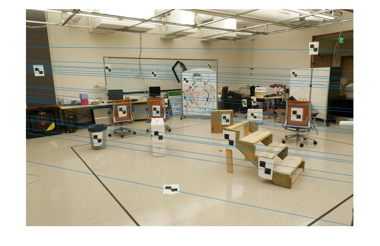
Result
The resulting fundamental matrix was
   -0.0000    0.0000   -0.0019
    0.0000    0.0000    0.0172
   -0.0009   -0.0264    0.9995
The epipolar lines look like this:

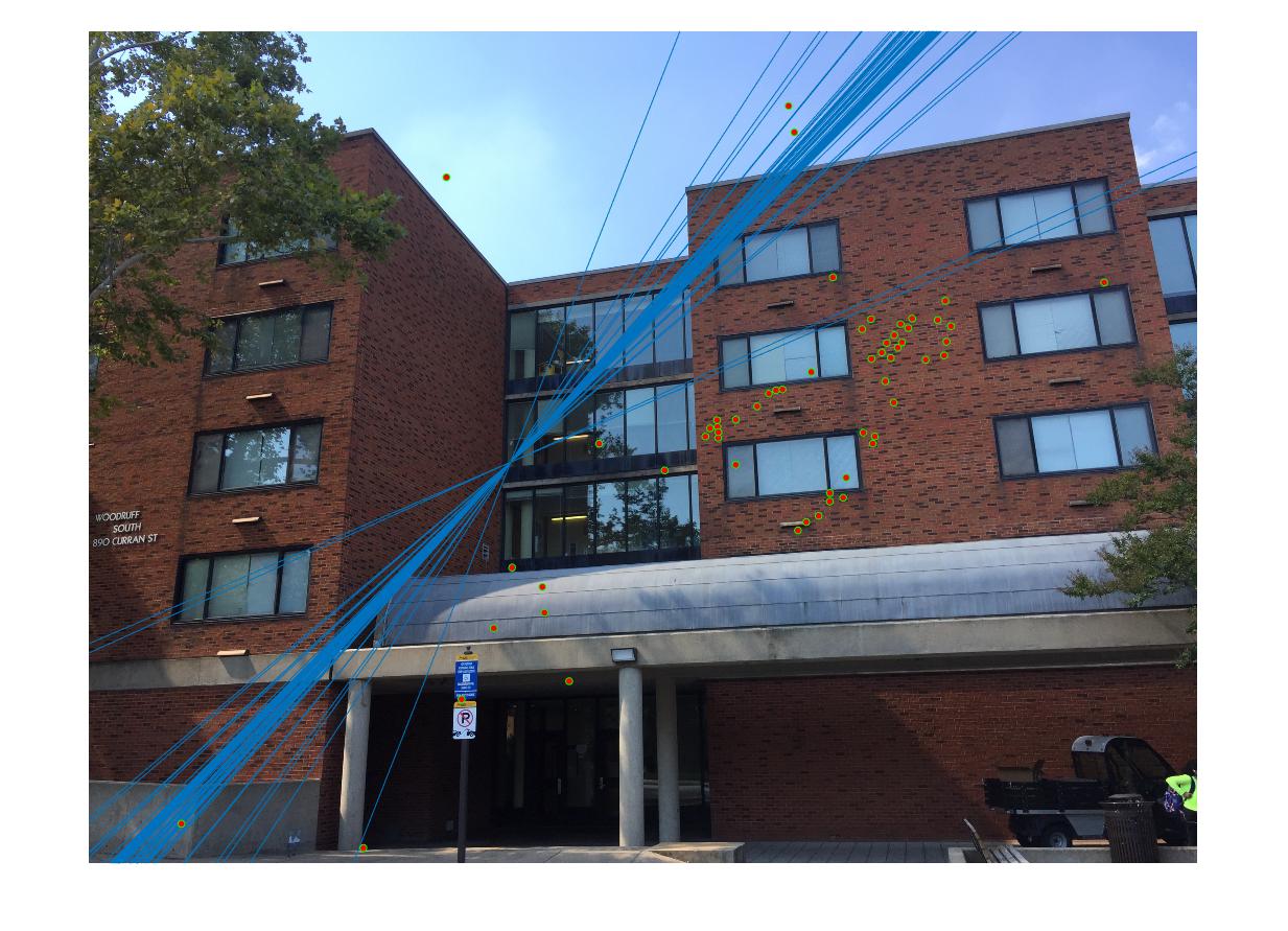
Part III: Fundamental Matrix with RANSAC
I used RANSAC in conjuction with SIFT to find a better fundamental matrix than in part 2. First SIFT finds many (several thousand) potential pairs of corresponding points between the two images. Next, RANSAC is used to find a good fundamental matrix for the points. A random set of 8 correspondences is chosen and used to estimate a fundamental matrix with the method developed in part 2. Next, the number of inlier correspondences is counted. An inlier is chosen if xFx' is close enough to zero, within some threshold. I chose a threshold of .0025 meaning that if xFx' >= .0025, then it is an outlier. 1000 random potential fundamental matrices are evaluated. The fundamental matrix F that resulted in the most inliers was chosen as the best fundamental matrix. Trying more than 1000 matrices did not improve results. The code for RANSAC looks like this:
numMatches = size(matches_a, 1);
indices = [1:numMatches];
error_threshold = .0025;
most_inliers = -1;
for i = 1:1000
    % randomly sample the number of points required to fit the model
    sampleIndices = randsample(indices, 8);
    matches_a_sample = matches_a(sampleIndices, :);
    matches_b_sample = matches_b(sampleIndices, :);
    % solve for model parameters using samples
    fun_matrix = estimate_fundamental_matrix(matches_a_sample, matches_b_sample); % XD
    % score the model by the fraction of inliers within a preset threshold
    % of the model
    current_inliers_a = [];
    current_inliers_b = [];
    num_inliers = 0;
    for row = 1:size(matches_a, 1)
        x = matches_a(row,:);
        x_prime = matches_b(row,:);
        match_error = abs([x 1] * fun_matrix * [x_prime 1]');
        if match_error < error_threshold
            num_inliers = num_inliers + 1;
            current_inliers_a = [current_inliers_a; x];
            current_inliers_b = [current_inliers_b; x_prime];
        end
    end
    if num_inliers > most_inliers
        Best_Fmatrix = fun_matrix;
        inliers_a = current_inliers_a;
        inliers_b = current_inliers_b;
        most_inliers = num_inliers;
    end
end
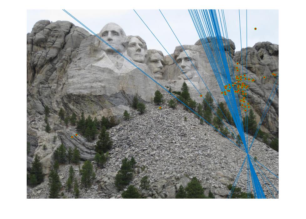
Results
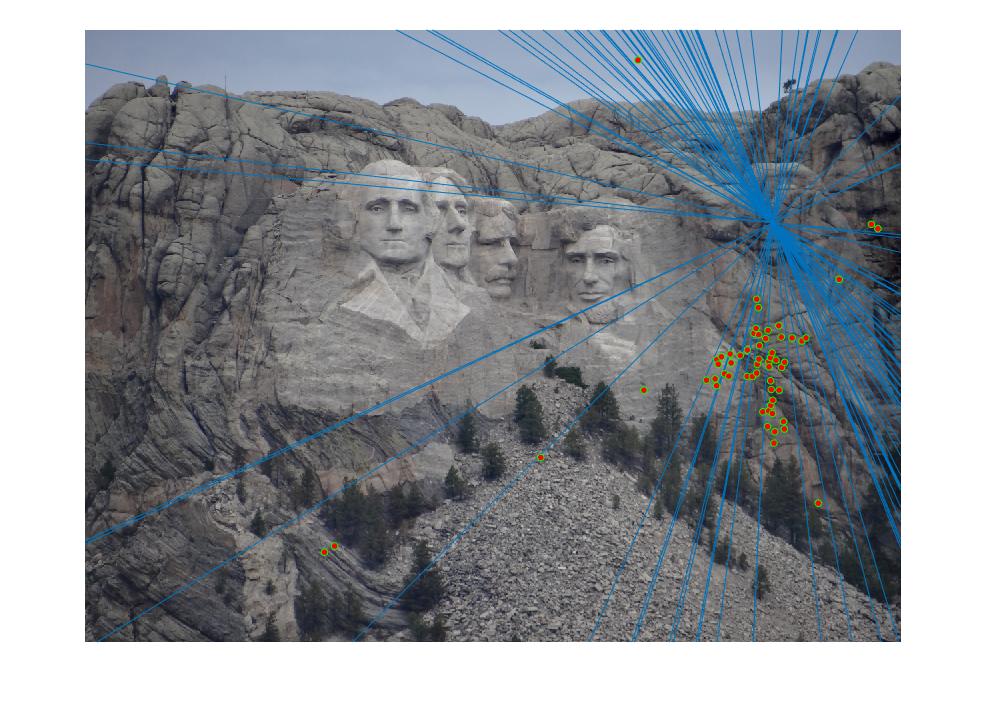
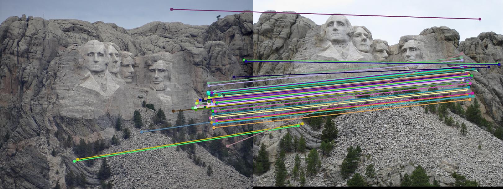
The Rushmore example did well with not many incorrect inliers and a fundamental matrix of
    0.0000    0.0000   -0.0005
    0.0000    0.0000   -0.0016
   -0.0006   -0.0014    1.0000
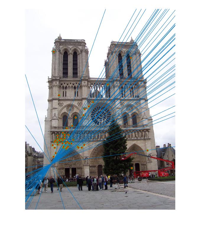
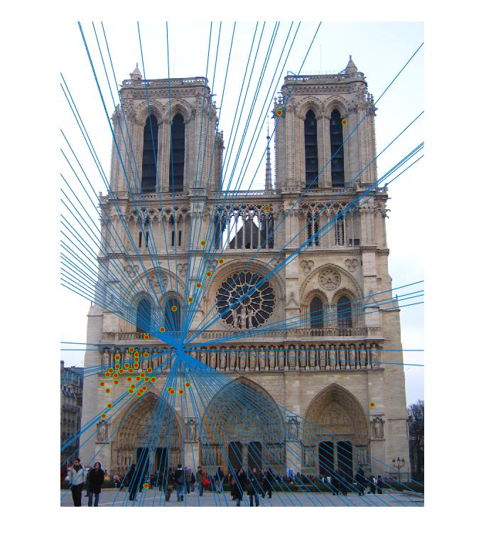
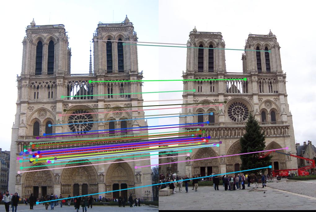
The Notre Dame example did well also with not many incorrect inliers and a fundamental matrix of
   -0.0000    0.0000   -0.0019
   -0.0000    0.0000   -0.0010
    0.0007   -0.0017    1.0000
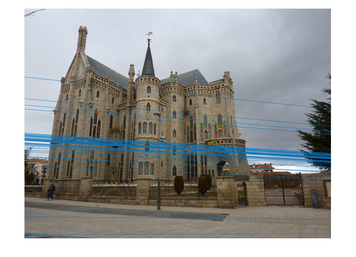
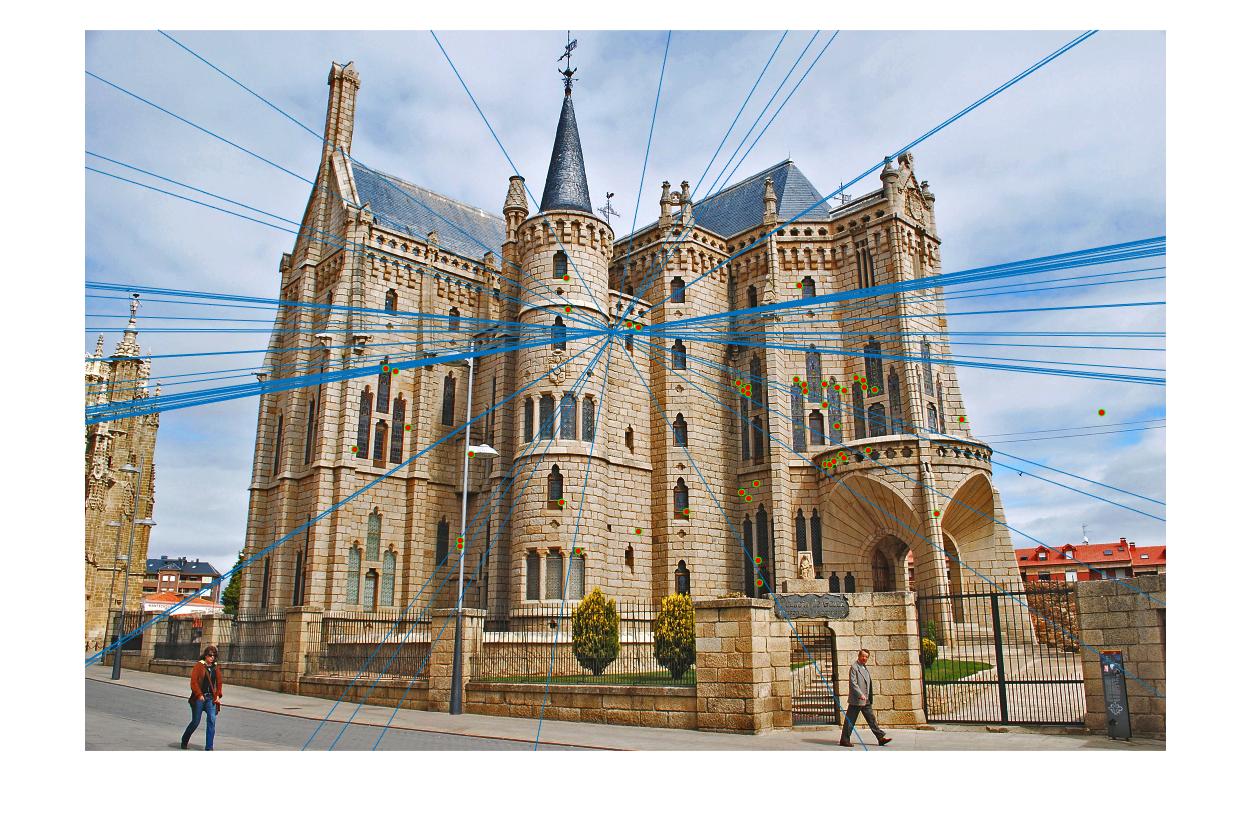
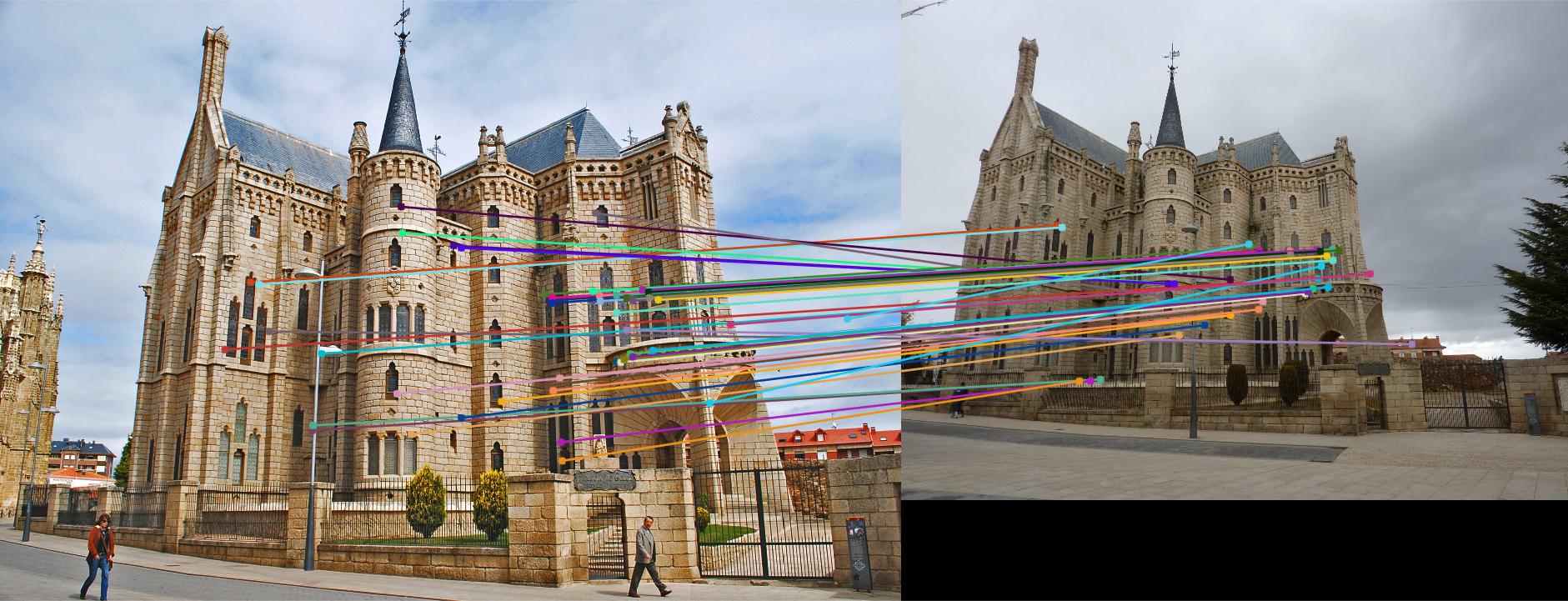
The Gaudi example did poorly with a good number of incorrect inliers and a fundamental matrix of
   -0.0000   -0.0000    0.0001
    0.0000    0.0000   -0.0015
   -0.0003   -0.0011    1.0000
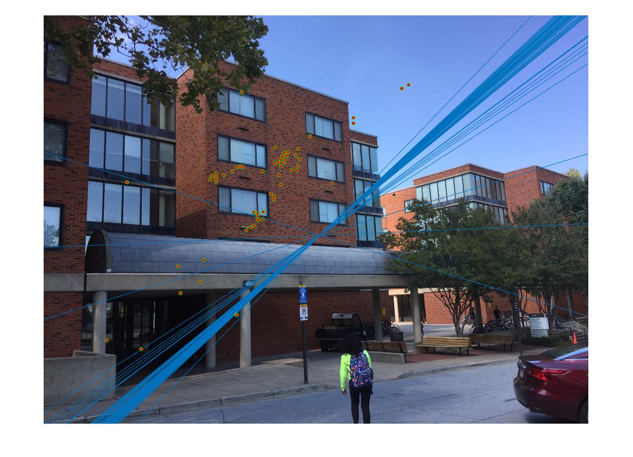
The Woodruff example did alright with a good number of correct inliers and a fundamental matrix of
    0.0000    0.0000   -0.0006
    0.0000    0.0000   -0.0006
   -0.0005   -0.0006    1.0000