Camera Projection Matrix
Method 1:
I have calculated the Camera Projection matrix from the normalized points using the homogeneous linear system of equations in calculate_projection_matrix.m. I used Singual Value Decomposition to compute the elements in the matrix. I obtained a scaled equivalent (here it is -1 times) of the desired result. I have also obtained the camera center
The projection matrix I obtained is:                      The actual projection matrix is:
    0.4583   -0.2947   -0.0140    0.0040                    -0.4583   0.2947   0.0139  -0.0040
   -0.0509   -0.0546   -0.5411   -0.0524                     0.0509   0.0546   0.5410   0.0524
    0.1090    0.1783   -0.0443    0.5968                    -0.1090  -0.1784   0.0443  -0.5968

The total residual is: <0.0445>
%%%
The estimated location of camera is:                      The actual location of camera is:
   <-1.5127, -2.3517, 0.2826>                                 <-1.5125, -2.3515, 0.2826>
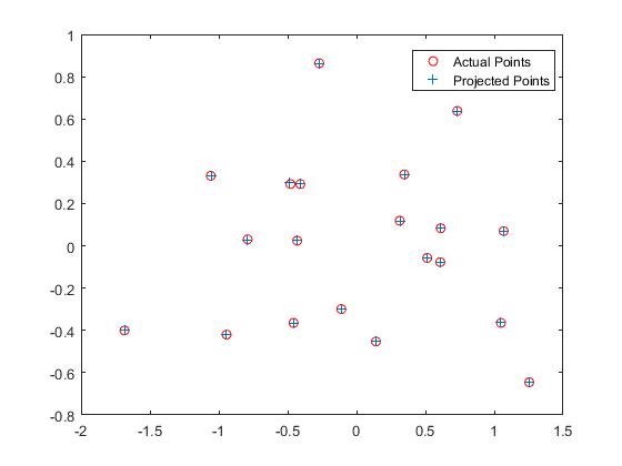
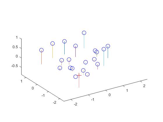
Now, using the projection matrix I obtained, here is an image (left one) of how well, the 3D points are projected into 2D points. They match very well. The right image shows the estimated location of the camera along with the 3D points.
	        %Code for the Calculation of the Projection Matrix:
		...
		...
		% obtaining the linear system of equations
		for i=1:size(Points_2D,1)
    		pr1 = -1*Points_3D(i,:)*Points_2D(i,1);
    		A = [A;Points_3D(i,:),one,zero,pr1,-1*one*Points_2D(i,1)];

    		pr2 = -1*Points_3D(i,:)*Points_2D(i,2);
    		A = [A;zero,Points_3D(i,:),one,pr2,-1*one*Points_2D(i,2)];

		end

		% solving the homogeneous linear system of equations using SVD
		[U, S, V] = svd(A);
		M = V(:,end);
		M = reshape(M, [], 3)';
    		...
    		...
Method 2:
I have also calculated the Camera Projection matrix from the normalized points using the non-homogeneous linear system of equations by setting the last element to 1 and then solving it using linear least squares. I obtained a scaled equivalent (here it is -0.5968 times) of the desired result. I have also obtained the camera center and the results are pretty similar to the above SVD method used for calculation
The projection matrix I obtained is:                      The actual projection matrix is:
    0.7679   -0.4938   -0.0234    0.0067                    -0.4583   0.2947   0.0139  -0.0040
   -0.0852   -0.0915   -0.9065   -0.0878                     0.0509   0.0546   0.5410   0.0524
    0.1827    0.2988   -0.0742    1.0000                    -0.1090  -0.1784   0.0443  -0.5968

The total residual is: <0.0445>

The projection matrix I obtained after scaling it accordingly:
   -0.4583    0.2947    0.0140   -0.0040
    0.0509    0.0546    0.5410    0.0524
   -0.1090   -0.1783    0.0443   -0.5968
%%%
The estimated location of camera is:                      The actual location of camera is:
   <-1.5126, -2.3517, 0.2827>                                 <-1.5125, -2.3515, 0.2826>
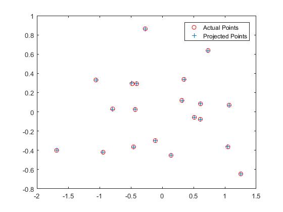
Now, using the projection matrix I obtained through this method, here is an image (left one) of how well, the 3D points are projected into 2D points. They match very well. The right image shows the estimated location of the camera along with the 3D points.
	        %Code for the Calculation of the Projection Matrix:
		...
		...
		%obtaining the linear system of equations
		for i=1:size(Points_2D,1)
    		pr1 = -1*Points_3D(i,:)*Points_2D(i,1);
    		A = [A;Points_3D(i,:),one,zero,pr1];

    		pr2 = -1*Points_3D(i,:)*Points_2D(i,2);
    		A = [A;zero,Points_3D(i,:),one,pr2];

    		Y = [Y,Points_2D(i,:)];
		end

		%solving the non-homogeneous linear system of equations using linear least squares
		Y=Y';
		M = A\Y;
		M = [M;1];
		M = reshape(M, [], 3)';
    		...
    		...
Fundamental Matrix Estimation
I have calculated the Fundamental matrix using the homogeneous linear system of equations in estimate_fundamental_matrix.m. I used Singual Value Decomposition to compute the elements in the matrix. The least squares estimate of F is full rank however, the fundamental matrix is a rank 2 matrix. So, in order to reduce its rank, I again used SVD and resolved it. I have also tried obtaining the same result by scaling the matrix and obtaining the solution using linear least squares but since, the results were pretty same. They are not shown here. Also, in my code, I have taken a transpose of the matrix obtained after solving because, I did not follow the same convention of u,v and u',v' as mentioned on the project webpage. I took the opposite, so I had to transpose it to use it other functions of the original given code.
The Fundamental matrix I obtained is:
-5.36264198382450e-07	7.90364770858074e-06   -0.00188600204023572
 8.83539184115781e-06	1.21321685009947e-06	0.0172332901014493
-0.000907382264407756  -0.0264234649922038	0.999500091906704
%
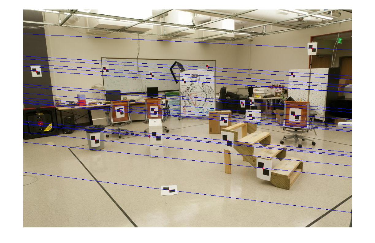
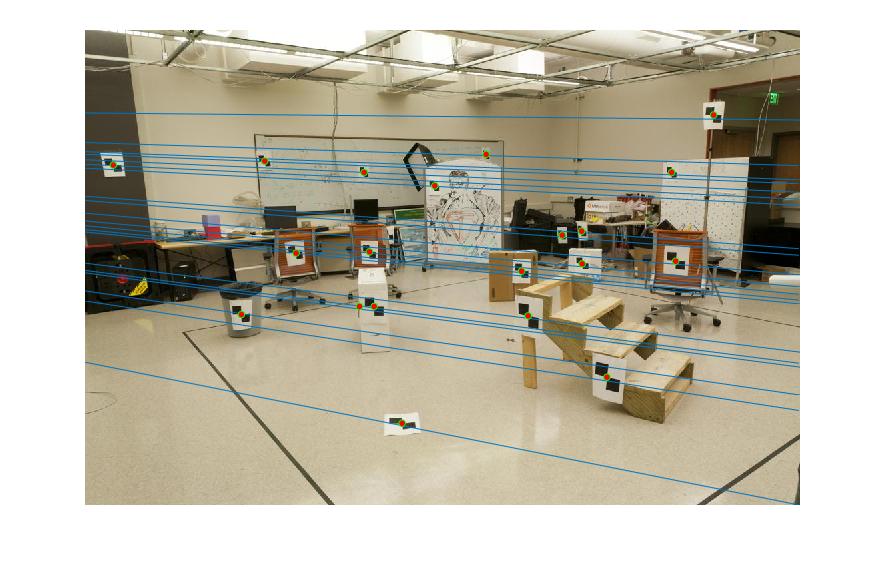
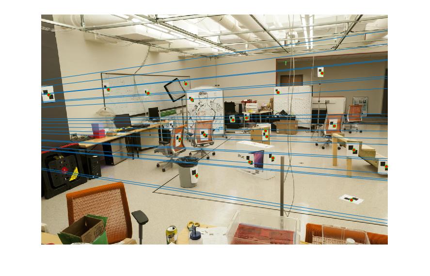
Using this fundamental matrix, following are the results of epipolar lines on both the images.
|
Image 1
|
Image 2
|
|
|
|
Image 1 with noise
|
Image 2 with noise
|
|

|
	        %Code for the Calculation of the Fundamental Matrix:
		...
		...
		% forming the linear system of equations.
		for i=1:size(Points_a,1)
    		A=[A;Points_a(i,1)*Points_b(i,1), Points_a(i,1)*Points_b(i,2), Points_a(i,1),
    				Points_a(i,2)*Points_b(i,1), Points_a(i,2)*Points_b(i,2), Points_a(i,2),
    					Points_b(i,1), Points_b(i,2), 1];
		end

		% using SVD to obtain the solution
		[U, S, V] = svd(A);
		f = V(:, end);
		F = reshape(f, [3 3])';

		% to reduce the rank of F-matrix to 2
		[U, S, V] = svd(F);
		S(3,3) = 0;
		F_matrix = U*S*V';
		% transpose because I have assummed u,v and u',v' in the opposite sense as
		% mentioned on the project webpage.
		F_matrix=F_matrix';
    		...
    		...
Fundamental Matrix with RANSAC
I have estimated the Fundamental matrix as above but by using RANSAC to figure out the best Fundamental matrix in ransac_fundamental_matrix.m. The algorithm I used is explained below. I used the 8-point algorithm in conjunction with RANSAC.
1. Obtain the potential matches using the SIFT wrapper.
2. Sample 8 points every iteration. and these 8 points are used to calculate the fundamental matrix using SVD.
3. Find the number of inliers based on a threshold (I used 0.01 for all the images).
4. Iterate steps 2 and 3 for about 2000 iterations and return the F matrix with most no. of inliers. Sample about 30 inliers and return them as matched points. Now, these are used to visualize the epipolar lines.
	        %Code for the Calculation of the Fundamental Matrix with RANSAC:
		...
		...
		for i=1:iterations
		    k=8;
		    inliers_a = zeros(0,size(matches_a,2));
		    inliers_b = zeros(0,size(matches_a,2));
		    ind = randperm(size(matches_a,1),k);
		    [ F_matrix ] = estimate_fundamental_matrix(matches_a(ind,:),matches_b(ind,:));
		    for j=1:size(matches_a,1)
		        % checking for potential matches
		        if abs([matches_b(j,:),1]*F_matrix*[matches_a(j,:),1]') < threshold
		            inliers_a = [inliers_a; matches_a(j,:)];
		            inliers_b = [inliers_b; matches_b(j,:)];
		        end
		    end
    		inliers = size(inliers_a,1);
    		if inliers > bestinliers % storing the best F_matrix and the inliers
        		bestinliers = inliers;
        		Best_Fmatrix = F_matrix;
        		bestinliers_a = inliers_a;
        		bestinliers_b = inliers_b;
    		end
		end

		display(bestinliers);
		% sampling random 30 inliers
		ind = randi(bestinliers,30,1);
		inliers_a = bestinliers_a(ind,:);
		inliers_b = bestinliers_b(ind,:);
    		...
    		...
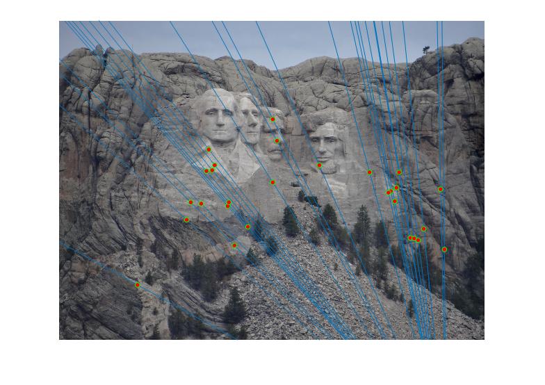
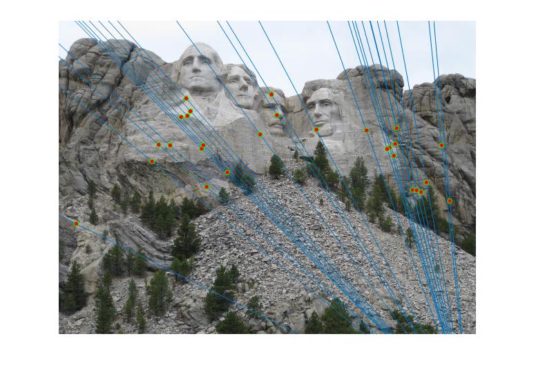
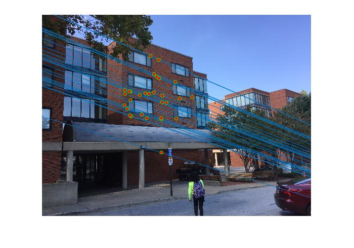
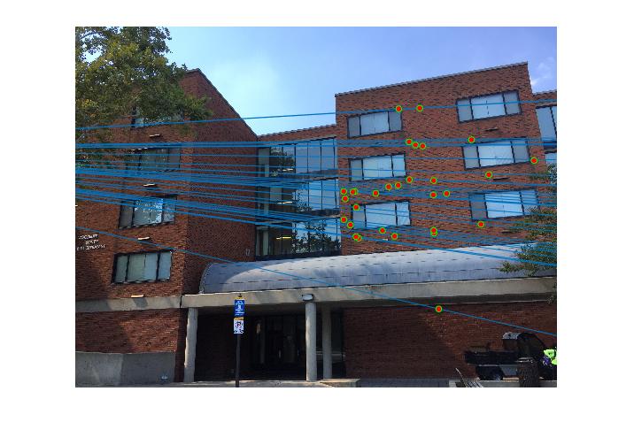
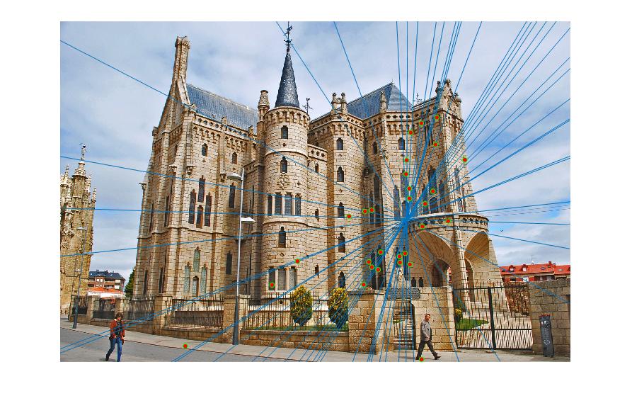
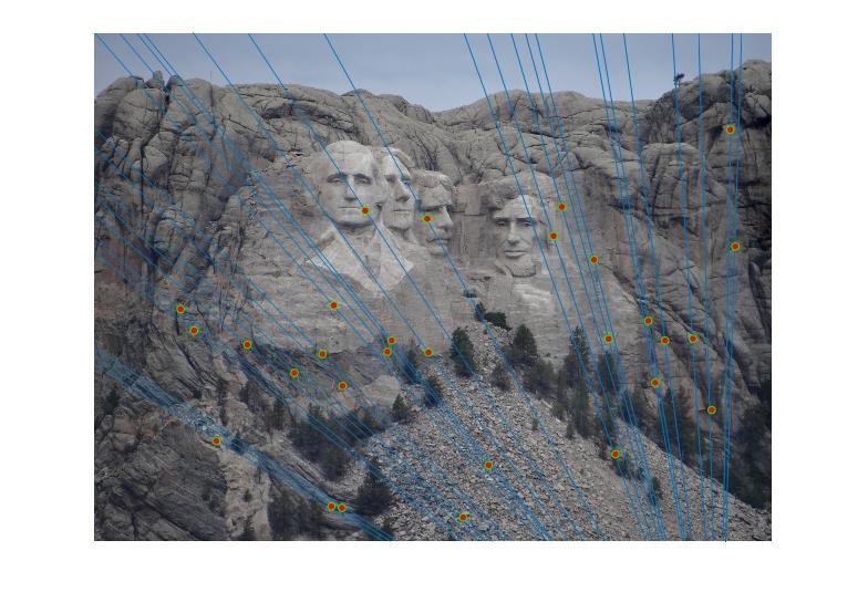
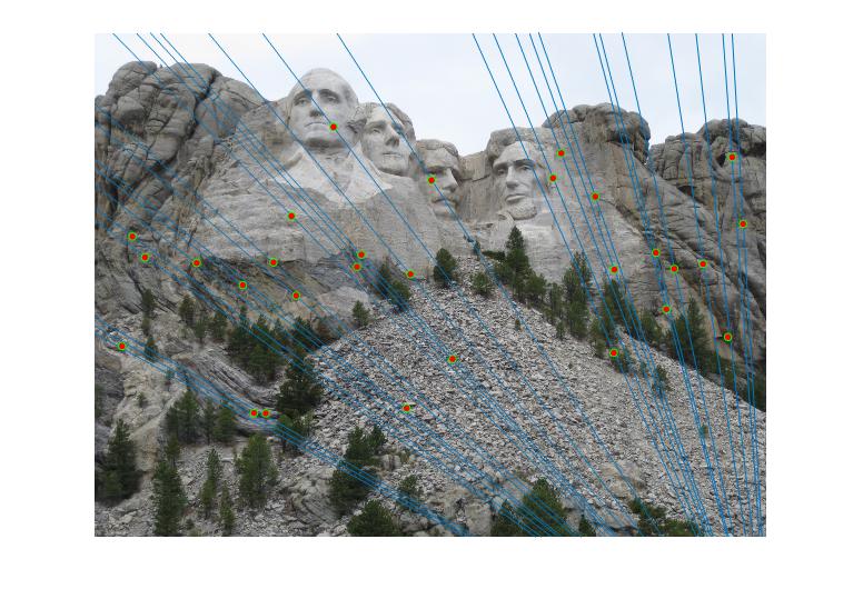
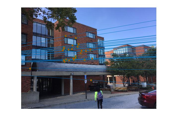
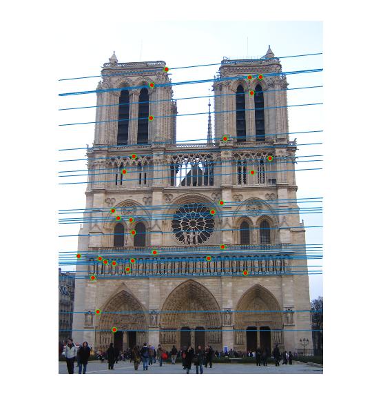
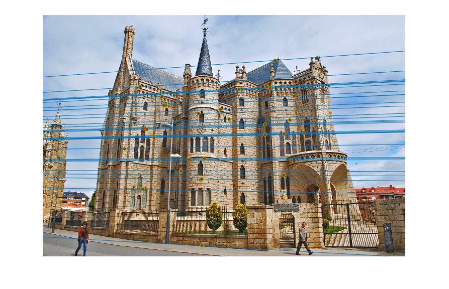
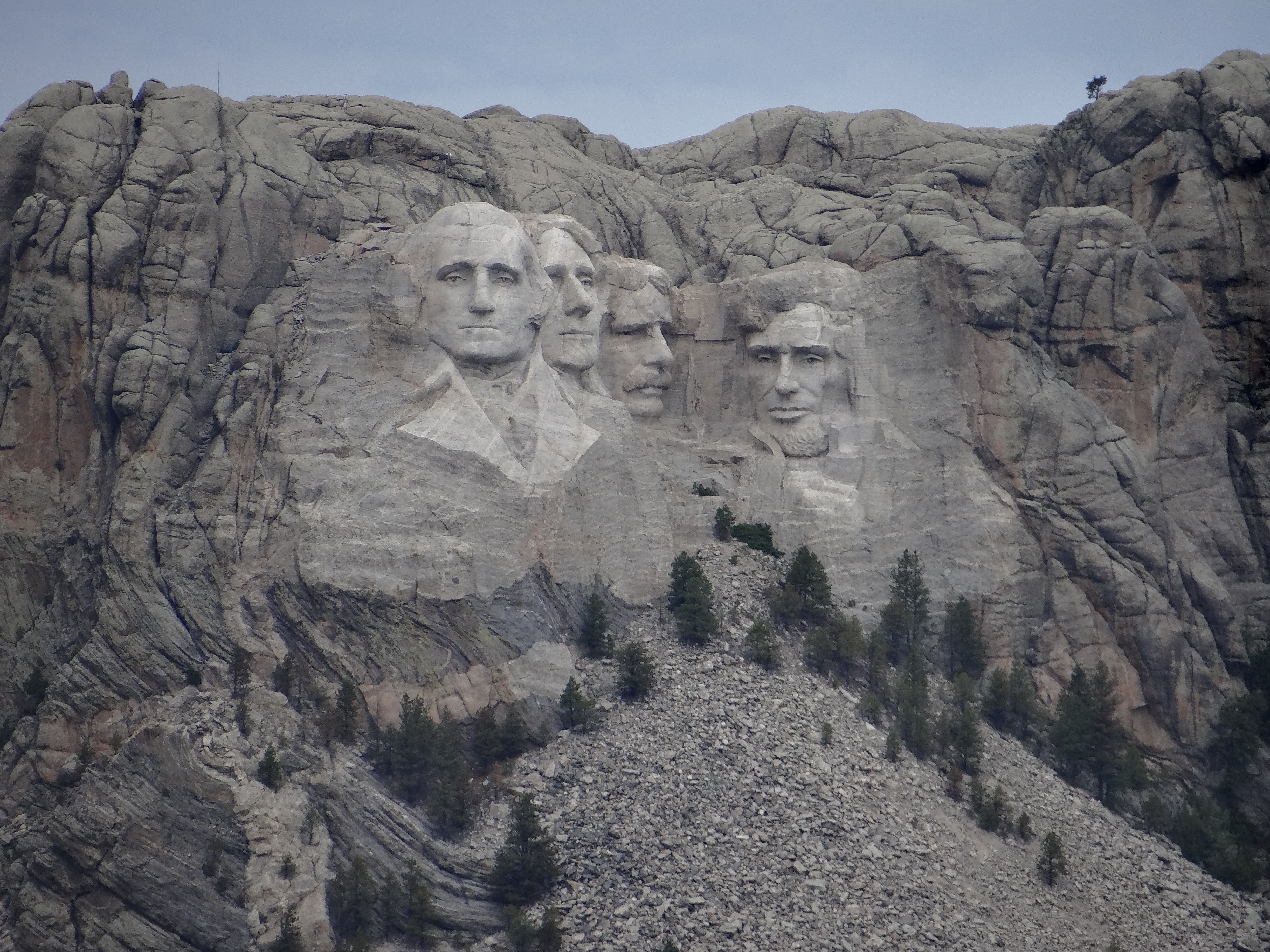
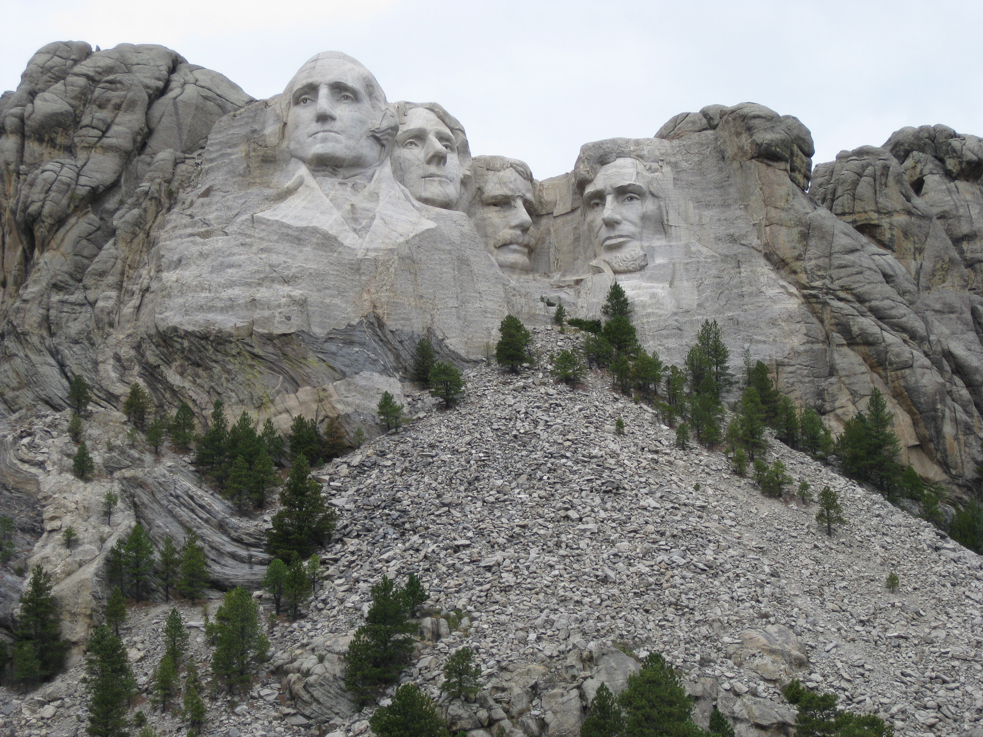
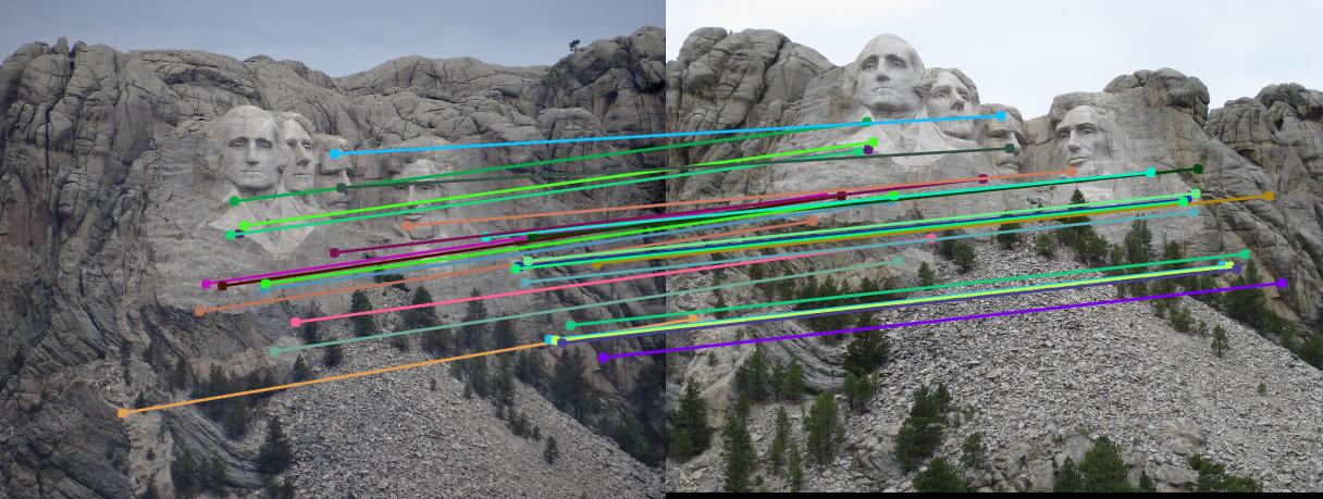
Below are the results of the images with inliers and also with epipolar lines. I sampled 30 points from the inliers and showed them for better visualization instead of showing all of the inliers. These are the results without normalization. Now, observe that most of the matches are correct in the results below except in the case of Episcopal Gaudi. It is later shown that normalization will help improve the performance.
Mount Rushmore
|
Image1
|
Image2
|
|
|
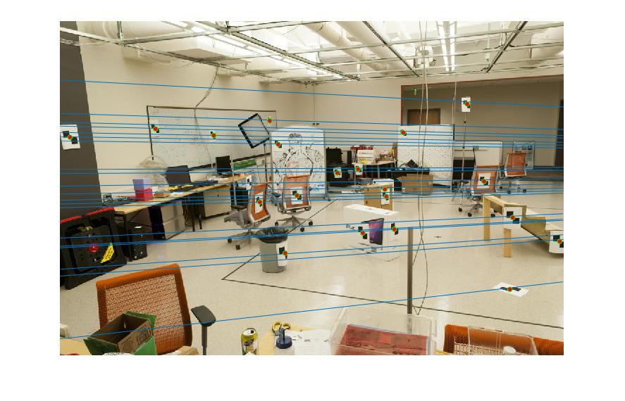
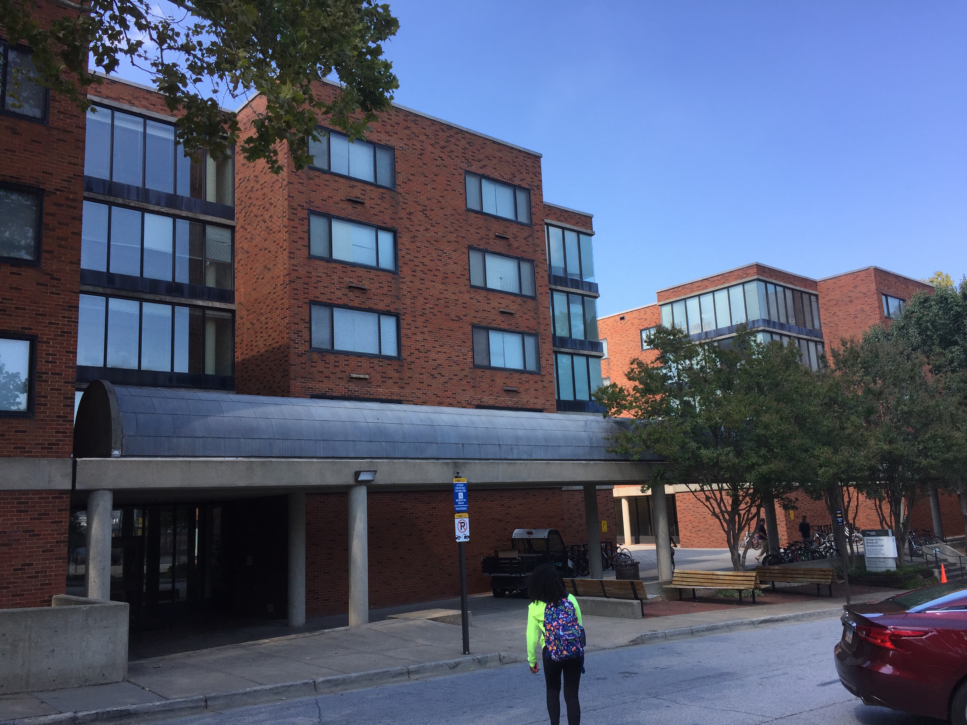
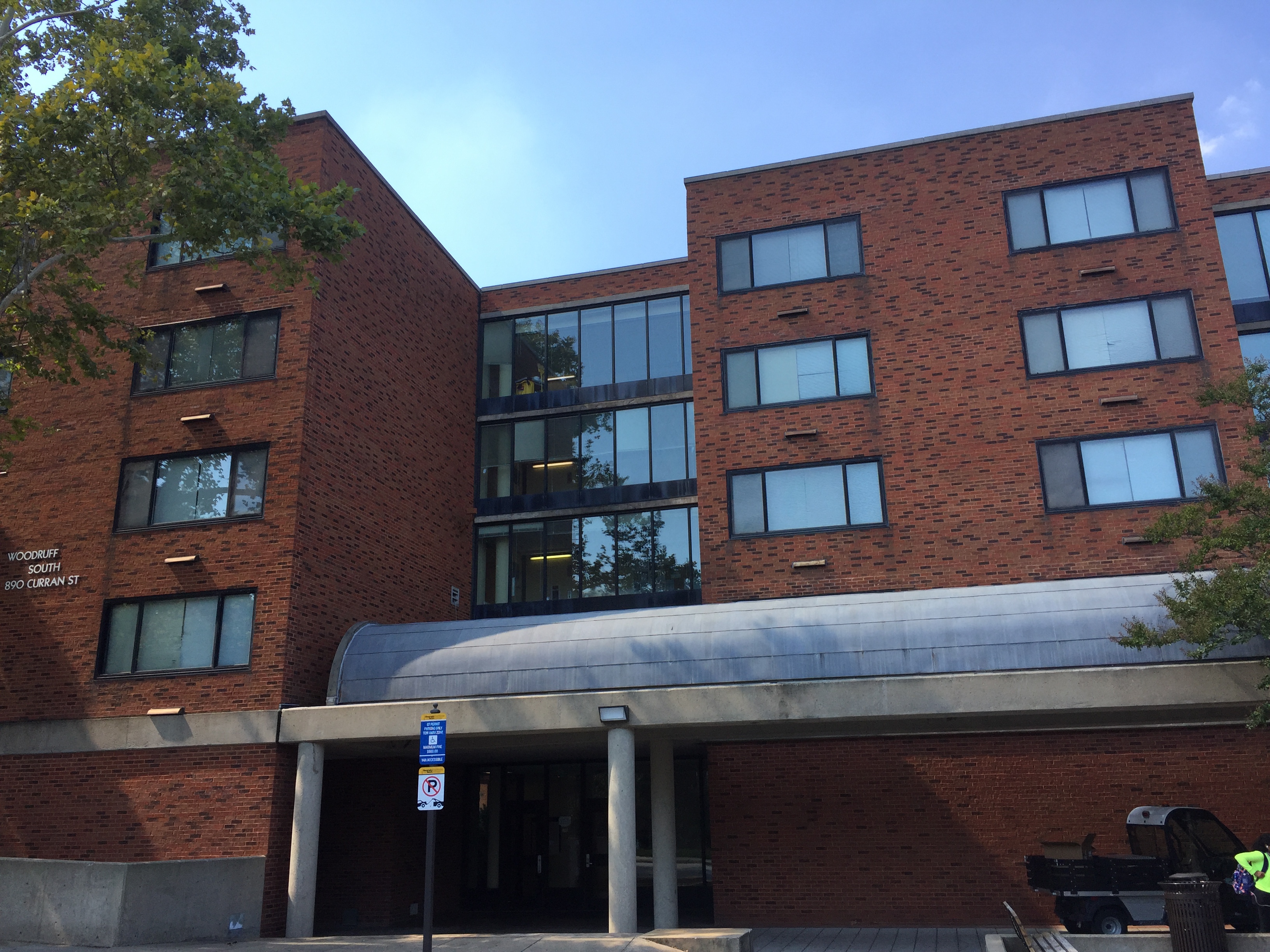
Woodruff Dorm
|
Image1
|
Image2
|
|
|
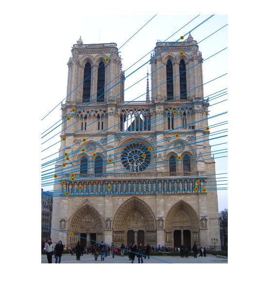
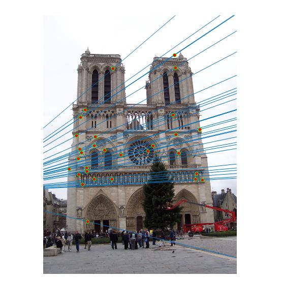
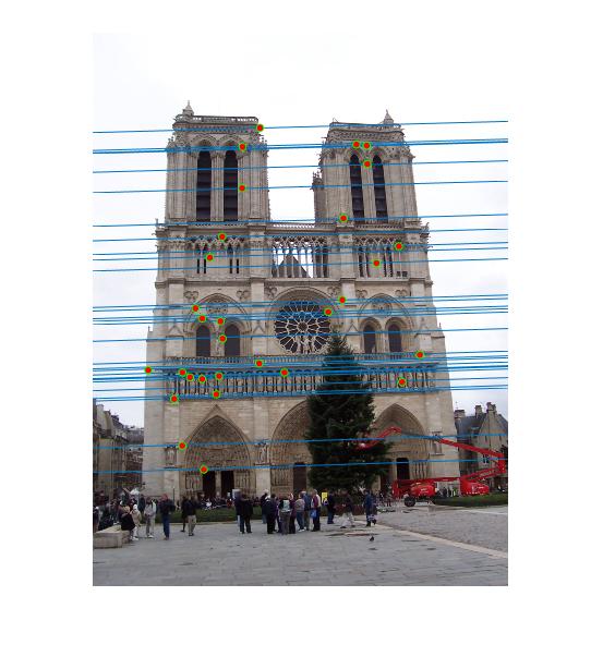
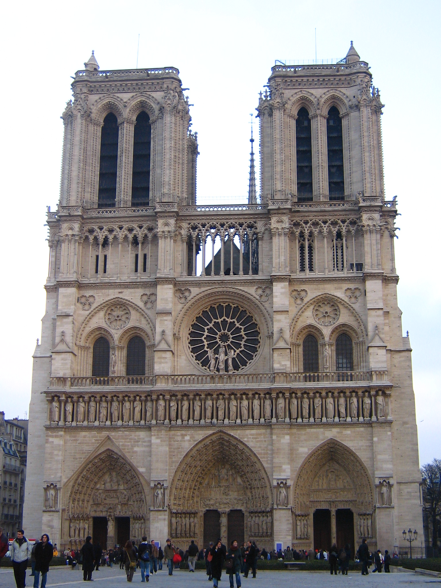
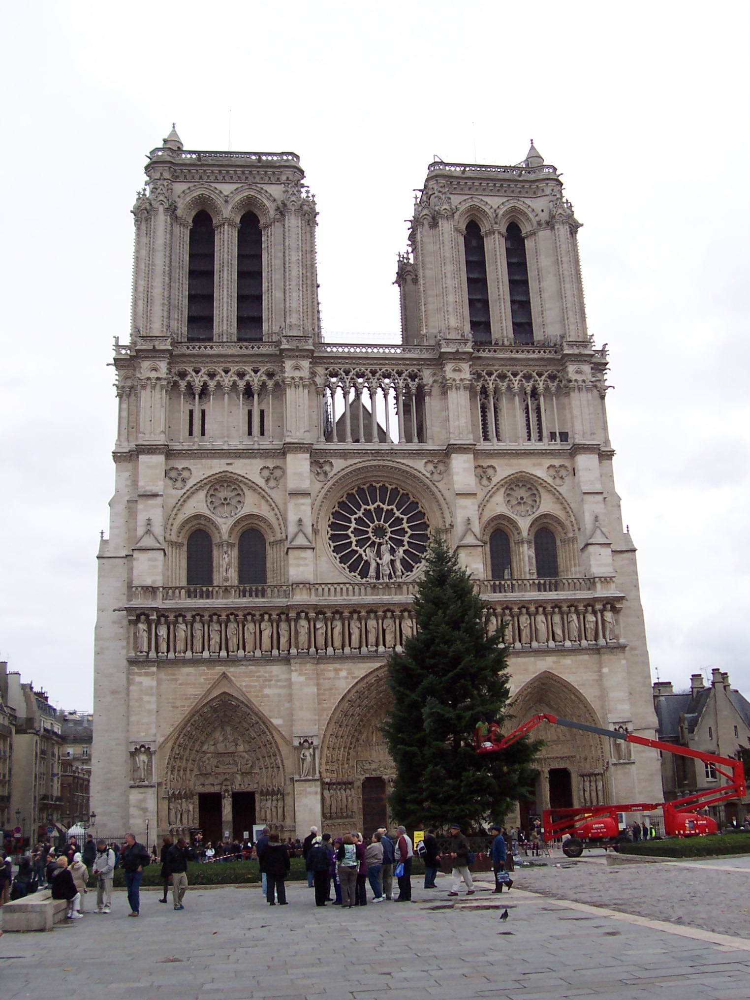
Notre Dame
|
Image1
|
Image2
|
|
|
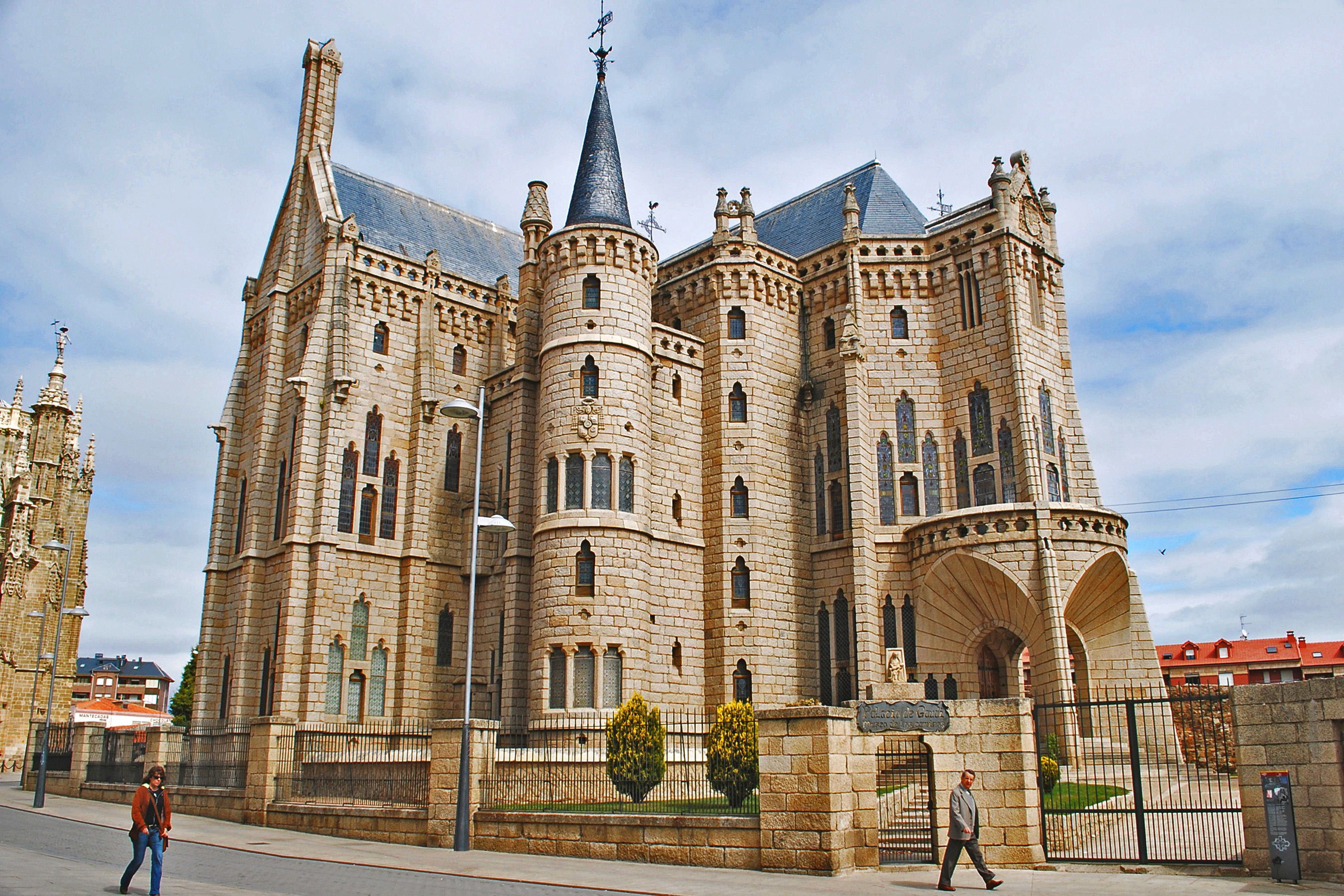
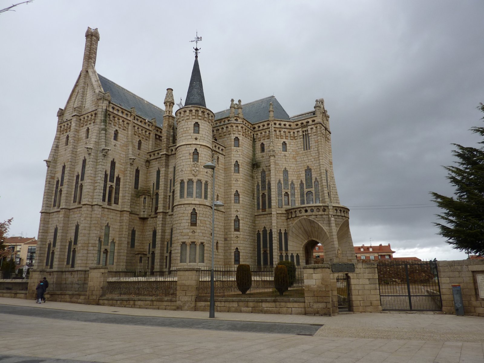
Episcopal Gaudi
|
Image1
|
Image2
|
|
|
Fundamental Matrix estimation using RANSAC with Normalization
I have implemented the part to normalize the points and then calculate the fundamental matrix. This is implemented in estimate_norm_fundamental_matrix.m In order to test this code, you need to change the file name in ransac_fundamental_matrix.m accordingly and then run the code. The steps I followed are as follows:
1. Sample about 8 match points from each image and send them to estimate_norm_fundamental_matrix.m
2. Obtain the mean of the these data points in each image and subtract the mean from the data points.
3. Now, obtain their standard deviation for along the x and y coordinates and use the inverse of this to find scale-x and scale-y and divide the co-ordinates of the data points respectively to normalize them.
4. Now, use these new points, and estimate the fundamental matrix as explained in Part II.
5. Use these mean and std-dev values to calculate the transformation matrix for each image and change the F matrix accordingly using the transformation matrix of both the images
6. Estimate the number of inliers (used 0.01 as threshold for all the images) as explained in Part III above and Use RANSAC for better estimation by repeating the above steps for about 2000 iterations and pick the best F matrix which gives the most number of inliers.
	        %Code for the Calculation of the Fundamental Matrix with RANSAC using normalized points:
		...
		...
		% normalizing the match_points_a
		matches_a = Points_a; ind = 1:size(matches_a,1); ind=ind';
		amatches = matches_a(ind,:);
		% finding mean and subtracting the data points
		amean = sum(amatches)/size(ind,1);
		amean = repmat(amean,size(ind,1),1);
		astd = std(matches_a(ind,:));
		amatches = amatches - amean;
		% finding std and dividing the data points
		amatches(:,1) = amatches(:,1)/astd(1); amatches(:,2) = amatches(:,2)/astd(2);
		transform_a = [1/astd(1),0,0; 0,1/astd(2),0; 0,0,1]*[1,0,-1*amean(1,1); 0,1,-1*amean(1,2); 0,0,1];

		% normalizing the match_points_b
		matches_b = Points_b; ind = 1:size(matches_b,1); ind=ind';
		bmatches = matches_b(ind,:);
		% finding mean and subtracting the data points
		bmean = sum(bmatches)/size(ind,1);
		bmean = repmat(bmean,size(ind,1),1);
		bstd = std(matches_b(ind,:));
		bmatches = bmatches - bmean;
		% finding std and dividing the data points
		bmatches(:,1) = bmatches(:,1)/bstd(1); bmatches(:,2) = bmatches(:,2)/bstd(2);
		transform_b = [1/bstd(1),0,0; 0,1/bstd(2),0; 0,0,1]*[1,0,-1*bmean(1,1); 0,1,-1*bmean(1,2); 0,0,1];

		Points_a = amatches;
		Points_b = bmatches;

		one = ones(1,1);
		parameters=9;
		A = zeros(0,parameters);

		for i=1:size(Points_a,1)
		    A=[A;Points_a(i,1)*Points_b(i,1), Points_a(i,1)*Points_b(i,2), Points_a(i,1),
		    	Points_a(i,2)*Points_b(i,1), Points_a(i,2)*Points_b(i,2),
		    		Points_a(i,2), Points_b(i,1), Points_b(i,2), 1];
		end

		[U, S, V] = svd(A);
		f = V(:, end);
		F = reshape(f, [3 3])';
		%F_matrix = F;

		[U, S, V] = svd(F);
		S(3,3) = 0;
		nF_matrix = U*S*V';
		normF_matrix=nF_matrix';

		% transforming the fundamental matrix back to work with original co-ordinates
		F_matrix = transform_b'*normF_matrix*transform_a;
    		...
    		...
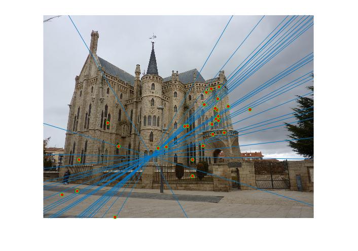
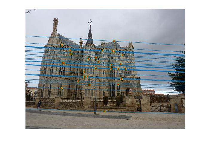
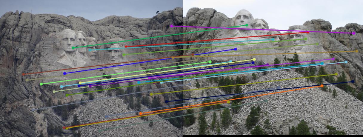
Below are the results of the images with about 30 randomly sampled inliers and also with epipolar lines. I sampled 30 points from the inliers and showed them for better visualization instead of showing all of the inliers. These are the results with normalization. Now, observe almost all the matches are correct in the results below. We also observe that normalization helps improve the performance in the case of Episcopal Gaudi.
Mount Rushmore
|
Image1
|
Image2
|
|
|
|
Woodruff Dorm
|
Image1
|
Image2
|
|
|
|
Notre Dame
|
Image1
|
Image2
|
|
|
|
Episcopal Gaudi
|
Image1
|
Image2
|
|
|
|
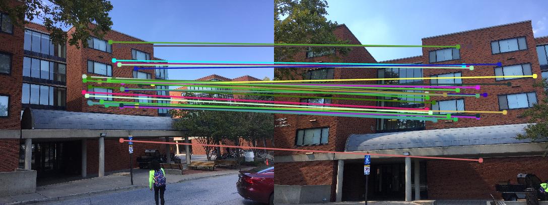
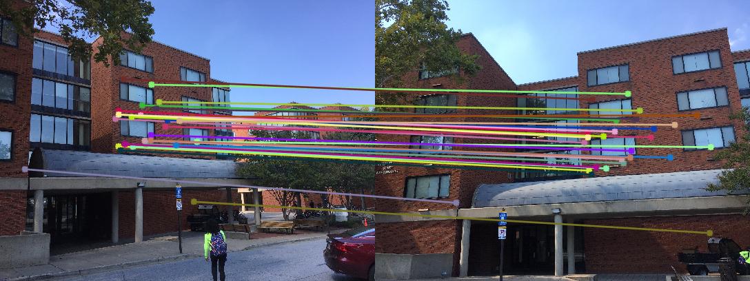
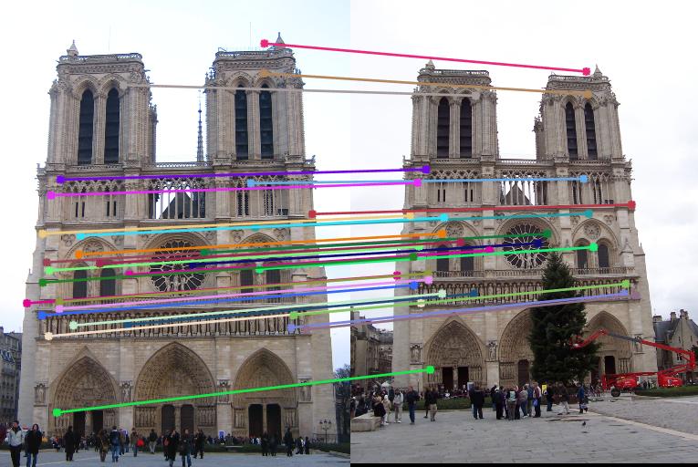
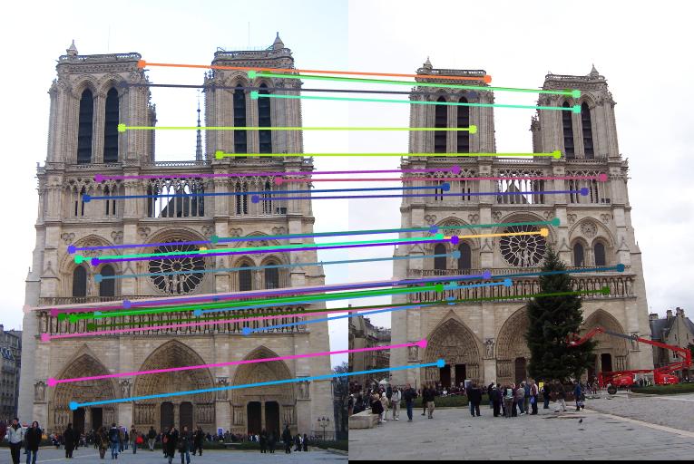
Comparison of Results with and without Normalization
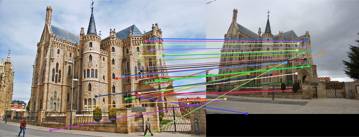
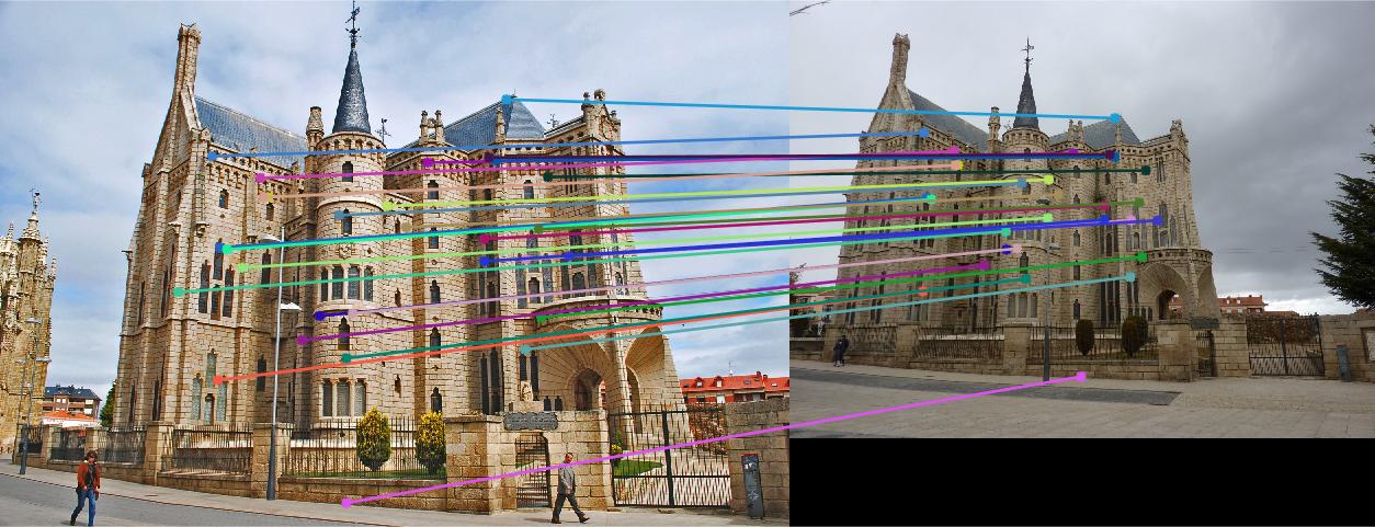
Below are the results of the images comparing the matches obtained with and without normalization of the points used for the calculation of the Fundamental matrix using RANSAC. Observe that using Fundamental matrix, we eliminate the spurious matches and obtain the matches which are most likely correct. Observing the Episcopal Gaudi pair, it is clear that normalization will help improve the performance as shown below.
Mount Rushmore
|
Result without Normalization
|
|
|
Result with Normalization
|
|
Woodruff Dorm
|
Result without Normalization
|
|
|
Result with Normalization
|
|
Notre Dame
|
Result without Normalization
|
|
|
Result with Normalization
|
|
Episcopal Gaudi
|
Result without Normalization
|
|
|
Result with Normalization
|
|
All the work that has been implemented for the project has been presented and discussed above. Feel free to contact me for further queries.
Contact details:
Murali Raghu Babu Balusu
GaTech id: 903241955
Email: b.murali@gatech.edu
Phone: (470)-338-1473
Thank you!