Project 3 / Camera Calibration and Fundamental Matrix Estimation with RANSAC
This projects consists of three parts each of which I will cover in its own section.Part I: Camera Projection Matrix
In the easy case of the normalized coordinates my camera matrix \(M\) and camera center \(C\) are equal to the solution given in the project description (up to sign). $$ M = \begin{pmatrix} 0.4583 & -0.2947 & -0.0140 & 0.0040\\ -0.0509 & -0.0546 & -0.5411 & -0.0524\\ 0.1090 & 0.1783 & -0.0443 & 0.5968 \end{pmatrix} \qquad C = \begin{pmatrix} -1.5127\\-2.3517\\0.2826 \end{pmatrix} $$ In the optional case without normalization I get the following matrix and center vector with a residual of \(15.5\). $$ M = \begin{pmatrix} 0.0069 & -0.0040 & -0.0013 & -0.8267\\ 0.0015 & 0.0010 & -0.0073 & -0.5625\\ 0.0000 & 0.0000 & -0.0000 & -0.0034 \end{pmatrix} \qquad C = \begin{pmatrix} 303.1000\\307.1843\\30.4217 \end{pmatrix} $$Part II: Fundamental Matrix Estimation
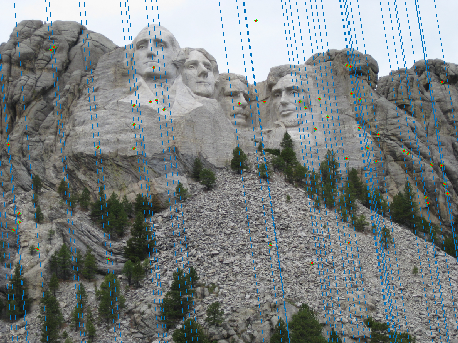
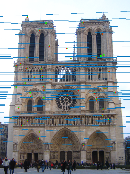
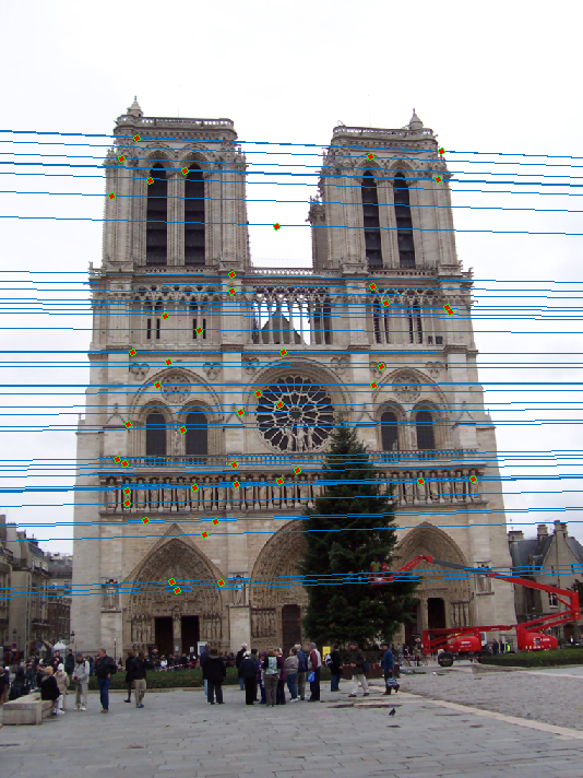
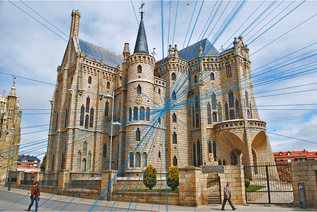
I get the following fundamental matrix $$ F = \begin{pmatrix} -0.0000 & 0.0000 & -0.0019\\ 0.0000 & 0.0000 & 0.0172\\ -0.0009 & -0.0264 & 0.9995 \end{pmatrix} $$ which produces these epipolar lines.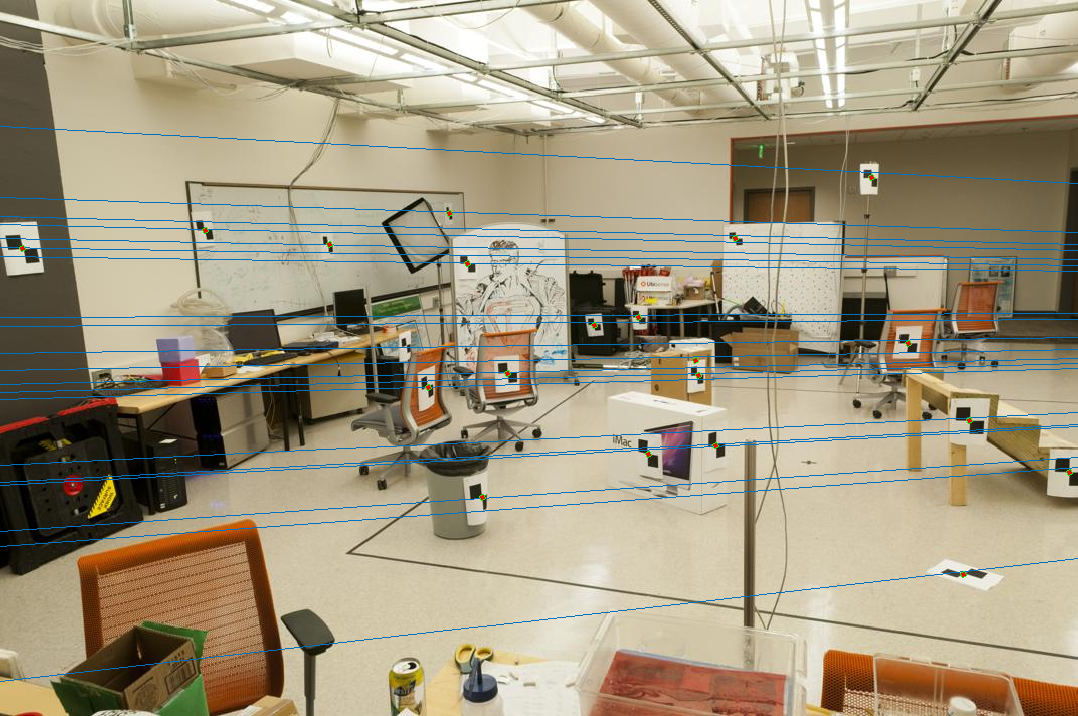
The epipolar lines are broadly correct though some of them miss the corresponding point by a few pixels. See the graduate credit section for improved results.
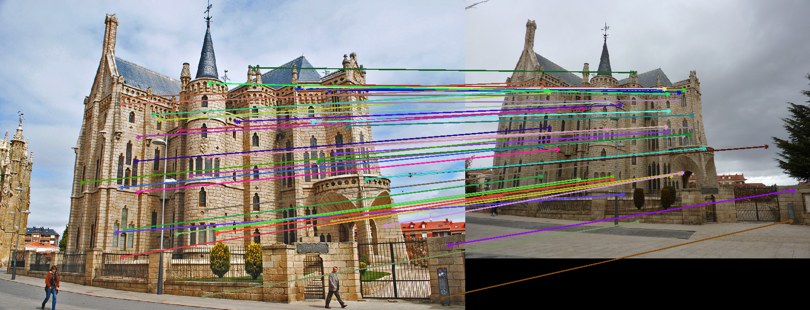
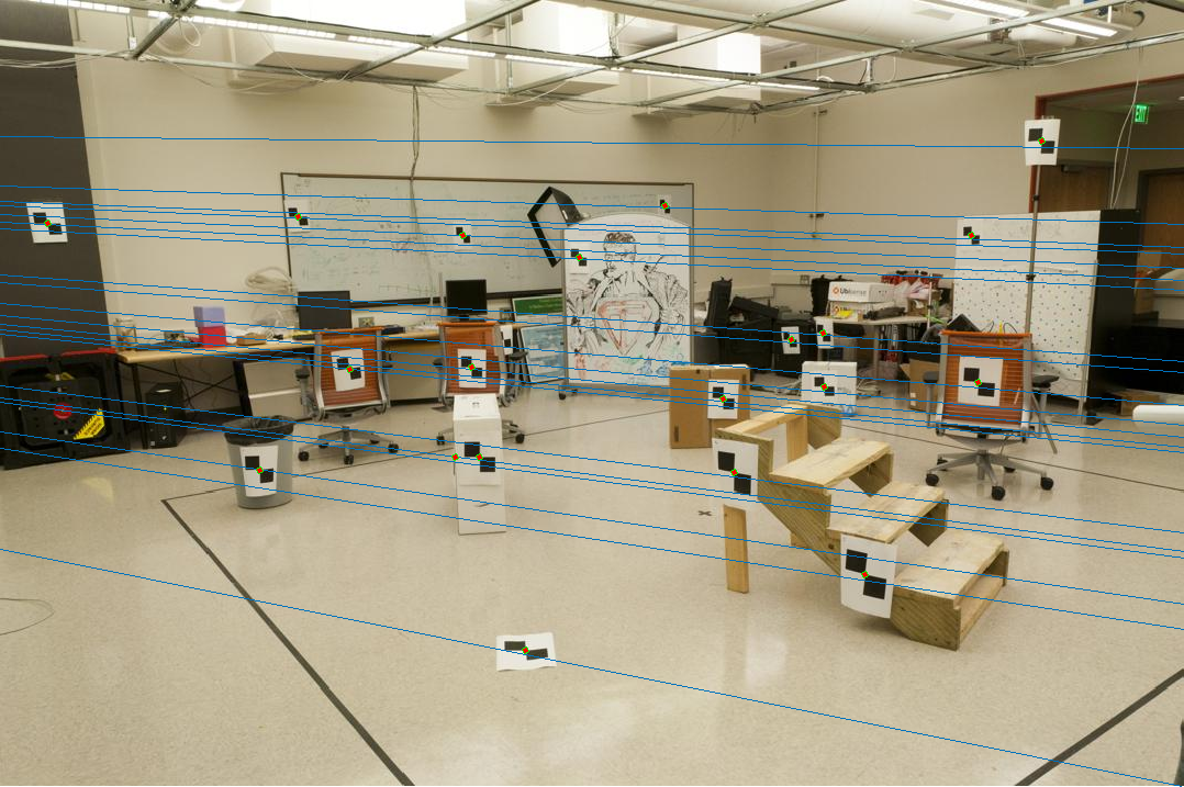
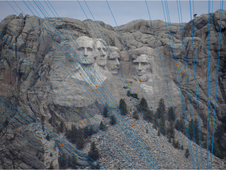
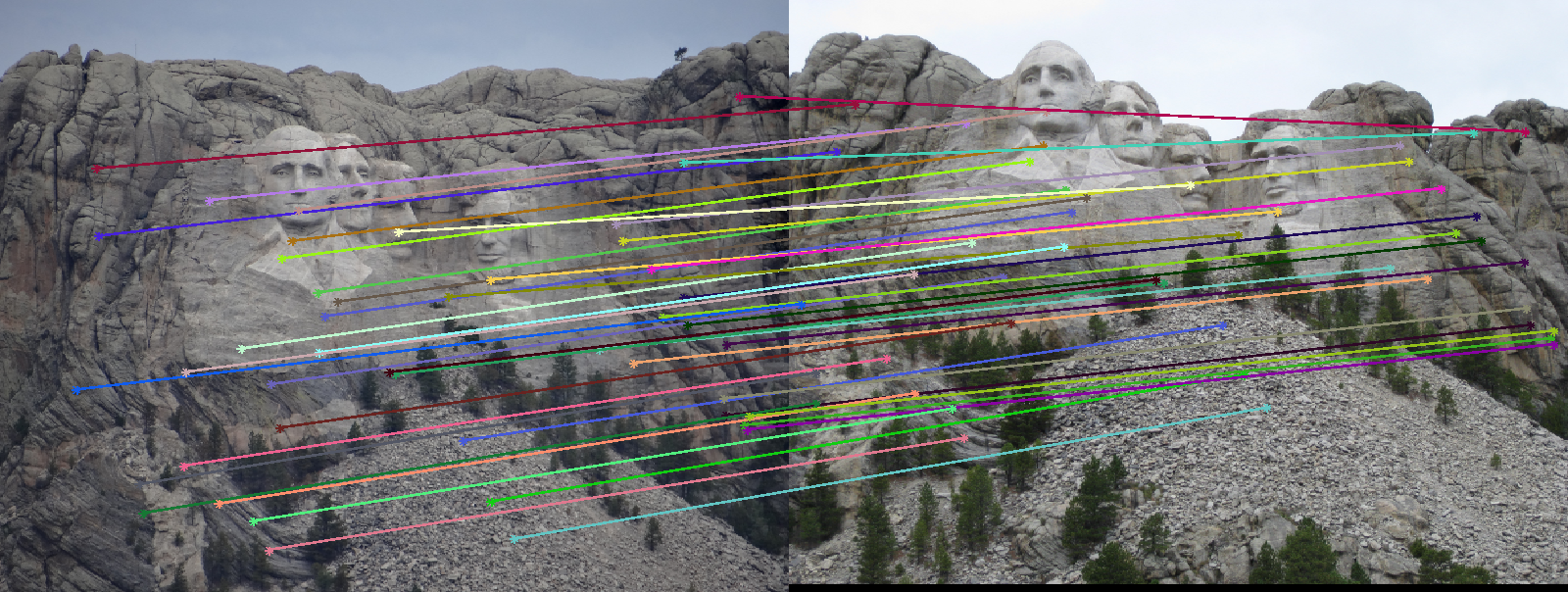
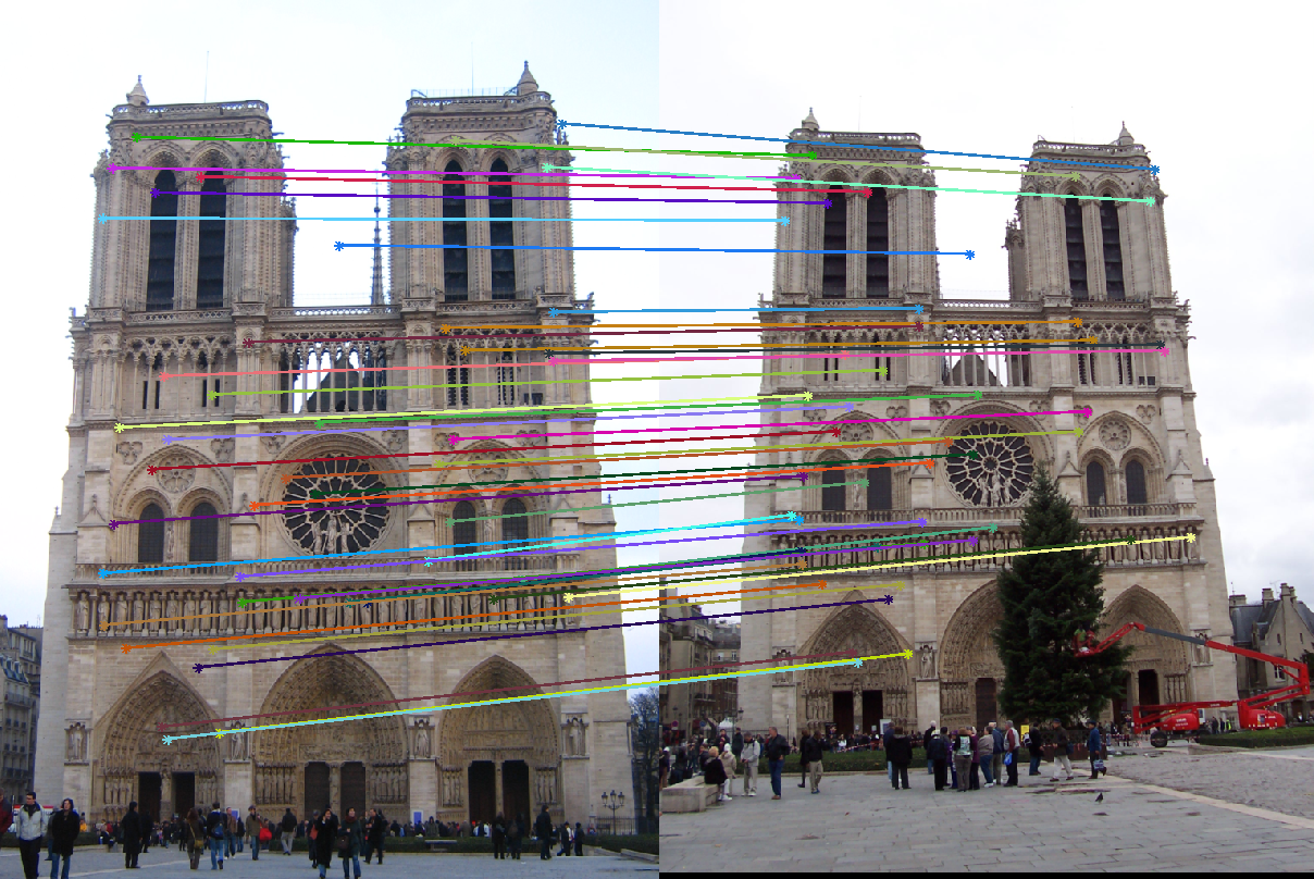
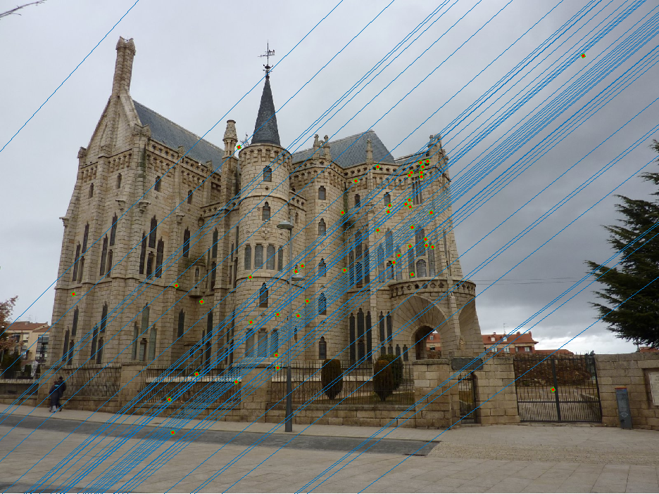
Part III: Fundamental Matrix with RANSAC
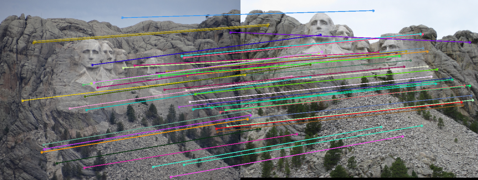
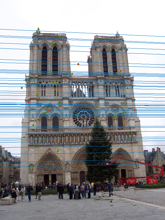
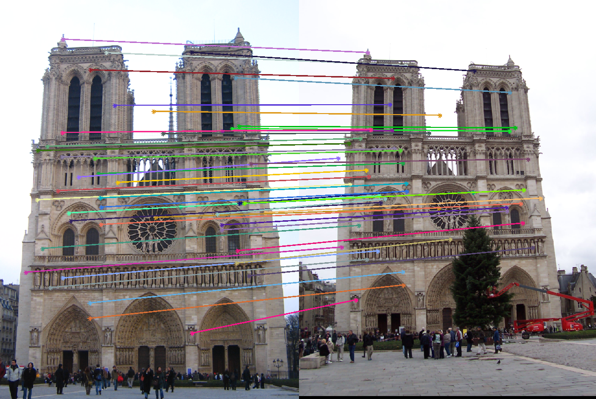
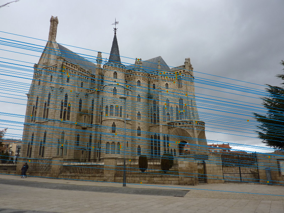
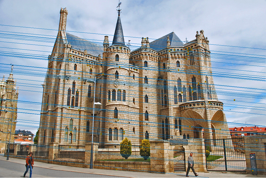
For part III I have implemented RANSAC on top of the fundamental matrix estimation from part II. In the following I present the resulting correspondences and epipolar lines I got for all three example pictures. For each case I have selected 45 inliers at random to show their correspondence and epipolar lines. The first two work very well, though due to the randomness it took a few tries to get such good results. The final picture of Gaudi's episcopal palace, however, did not budge and even though these matches are significantly better than what I achieved in the second project, they still contain a handful of mismatches in contrast to the first two pictures.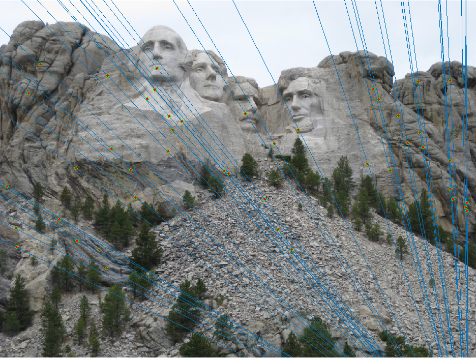

Graduate Credit
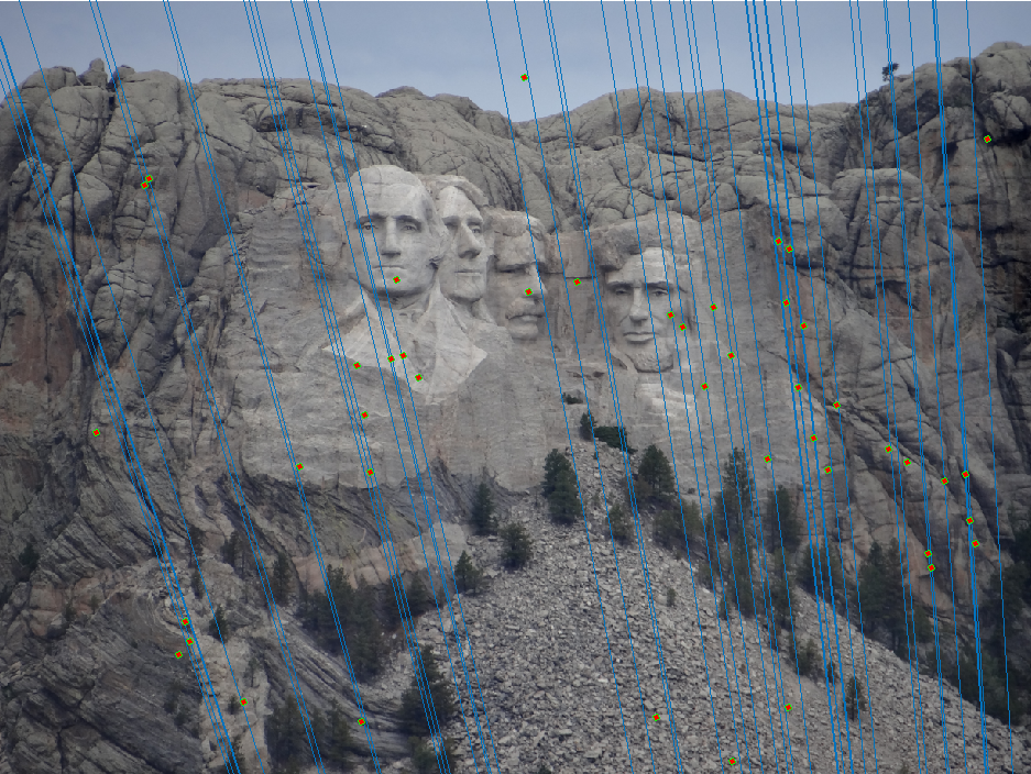
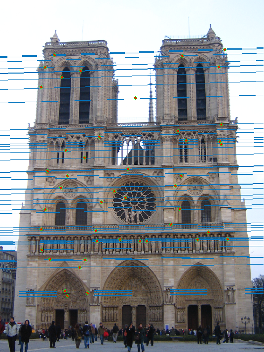
For graduate credit I implemented coordinate normalization. To have a case with ground-truth available, I began with a re-run of part II. This time I got the following fundamental matrix, which has similar structure as the \(F\) from part II but all elements are of lesser magnitude. $$ F = \begin{pmatrix} -0.0000 & 0.0000 & -0.0007\\ 0.0000 & -0.0000 & 0.0055\\ -0.0000 & -0.0075 & 0.1740 \end{pmatrix} $$
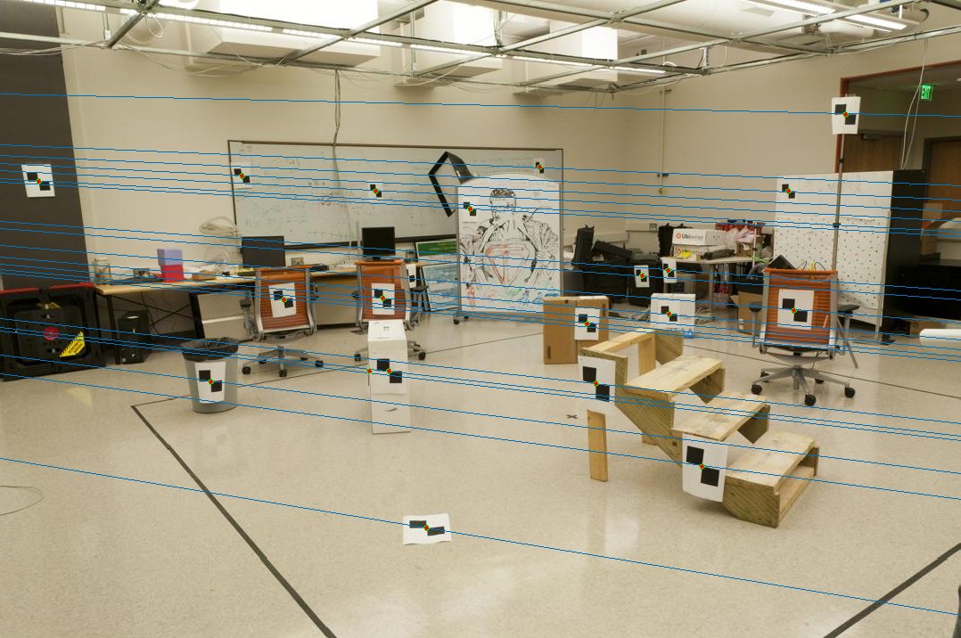
With coordinate normalization the epipolar lines are pixel-perfect.