Project 3: Scene Geometry and Model Fitting
Author: Mitchell Manguno (mmanguno3)
Table of Contents
- Table of Contents
- Synopsis
- Pt. 1: Camera Projection Matrix
- Pt. 2: Fundamental Matrix Estimation
- Pt. 3: Fundamental Matrix with RANSAC
Synopsis
For this project, principles of camera calibration and epipolar geometry were utilized to complete a SIFT-RANSAC pipeline for image matching. The project was seperated into three parts: (1) computation of the camera's projection matrix and camera center, (2) computation of the fundamental matrix and further calculation of the epipolar lines, and (3) utilizing SIFT and RANSAC to gather data for and test candidate fundamental matrices, until finding the 'best' one in order to reject keypoint matching outliers.
We begin the discussion with part 1, the camera projection matrix.
Pt. 1: Camera Projection Matrix
The camera projection matrix is the relation between 2D image coordinates and 3D world coordinates. It can be easily by found by solving a simple linear system of equations:
                                                   [M11       [ u1
                                                    M12         v1
                                                    M13         .
                                                    M14         .
[ X1 Y1 Z1 1 0  0  0  0 -u1*X1 -u1*Y1 -u1*Z1 ]       M21         .
| 0  0  0  0 X1 Y1 Z1 1 -v1*Z1 -v1*Y1 -v1*Z1 |       M22         .
| .  .  .  . .  .  .  .    .     .      .   |     * M23   =     .
| Xn Yn Zn 1 0  0  0  0 -un*Xn -un*Yn -un*Zn |       M24         .
[ 0  0  0  0 Xn Yn Zn 1 -vn*Zn -vn*Yn -vn*Zn ]       M31         .
                                                   M32         un
                                                   M33         vn ]
Where each Mi,j is a member of the camera projection matrix, X, Y, and Z are the world coordinates, and u and v are the image coordinates.
This can easily be solved in MATLAB, with it's linear equation solver.
% For each 2D -> 3D pair of points, calculate each row of 'A'.
% This will be done with two matrix multiplications per 2 rows (that is,
% two matrix operations per every 2D -> 3D pair), all to be concatenated
% into A.

n = size(Points_2D, 1);  % The number of points
A = zeros(2*n, 11);
j = 1;  % Need another looping variable that increments by 2

for i=1:n
    ui = Points_2D(i,1);
    vi = Points_2D(i,2);

    Xi = Points_3D(i,1);
    Yi = Points_3D(i,2);
    Zi = Points_3D(i,3);

    row_1 = [Xi, Yi, Zi, 1] * [eye(4) zeros(4) [diag([-ui, -ui, -ui]);[0,0,0]]];
    row_2 = [Xi, Yi, Zi, 1] * [zeros(4) eye(4) [diag([-vi, -vi, -vi]);[0,0,0]]];

    A(j,:)   = row_1;
    A(j+1,:) = row_2;
    j = j + 2;
end

% The RHS of the equation.
Y = reshape(Points_2D', [2*n,1]);

% Now, use the least squares to calculate M, the projection matrix.
% (Note: this code from lecture 13 slides, slide #37).
M = A\Y;
M = [M;1];
M = reshape(M,[],3)';
We then calculate the camera's center by seperating M into a matrix Q and a vector m4 :
% Let M = (Q | m_4). Then, C = -Q^-1 * m_4. (From proj3 instructions).
Q   = M(1:3, 1:3);
m_4 = M(1:3, 4);

Center = -inv(Q) * m_4;
When evaluated over the points given, we get the following results:
The projection matrix is:
    0.7679   -0.4938   -0.0234    0.0067
   -0.0852   -0.0915   -0.9065   -0.0878
    0.1827    0.2988   -0.0742    1.0000


The total residual is: <0.0445>

The estimated location of camera is: <-1.5126, -2.3517, 0.2827>
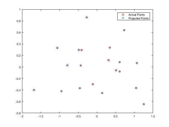
Visually, we can see that the points align quite well with our expectations:
 |
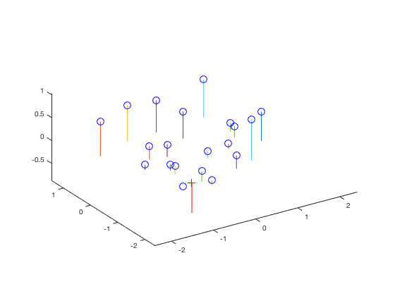 |
| fig. 1 Projected points vs. actual points | fig. 2 3D representation of the approximations |
Pt. 2: Fundamental Matrix Estimation
In the second part of the project, the fundamental matrix was calculated, which relates points in one image to lines in the other. Similar to the camera calibration matrix, we use a system of equations to find the fundamental matrix:
                                               [f1,1
                                                f1,2
[u1u1' u1v1' u1 v1u1' v1v1' v1 u1' v1' 1]         f1,3
|  .     .   .  .     .    .  .   .  .|      *  f2,1   =  0
[unun' unvn' un vnun' vnvn' vn un' vn' 1]         .
                                                .
                                                f3,3]
Where the f values represent the values of the fundamental matrix.
As our equation is now Af = 0, we can use the SVD to calculate a non-trivial solution:
for i=1:n
    ui = Points_b(i,1);
    vi = Points_b(i,2);

    ui_prime = Points_a(i,1);
    vi_prime = Points_a(i,2);

    A(i,:) = [ui*ui_prime, ui*vi_prime, ui, vi*ui_prime, vi*vi_prime,...
              vi, ui_prime, vi_prime, 1];

end

% Now, use an SVD to calculate F, the projection matrix.
% (Note: this code adapted from lecture 14 slides, slide #34).
[~, ~, V] = svd(A);
f = V(:, end);
F_matrix = reshape(f, [3 3])';
An additional requirement on F is this: it's determinant must equal zero. We can enforce this by reducing its rank via another SVD:
%% Now, resolve det(F) = 0 constraint using SVD
% (Note: this code from lecture 14 slides, slide #36).
[U, S, V] = svd(F_matrix);
S(3,3) = 0;
F_matrix = U*S*V';
When run on the test pictures, we get an F matrix like this:
F_matrix =

   -0.0000    0.0000   -0.0019
    0.0000    0.0000    0.0172
   -0.0009   -0.0264    0.9995
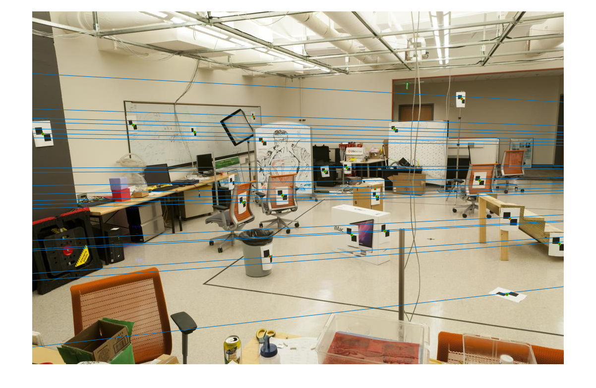
This F produces the following lines on the test images:
 |
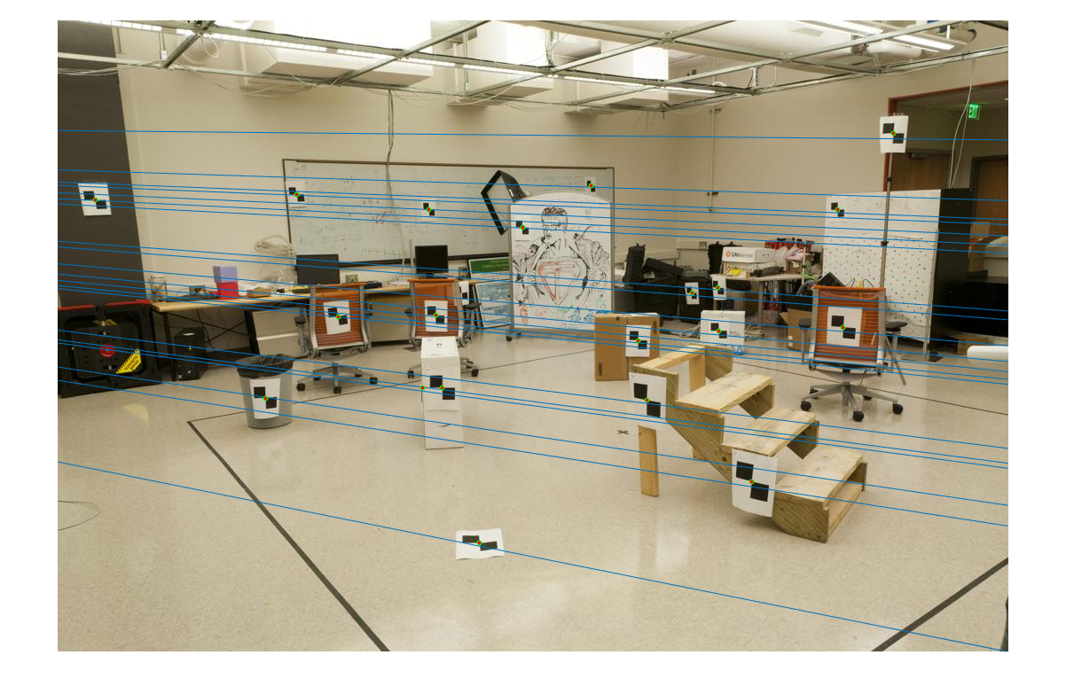 |
| fig. 3 epipolar lines in pic_a | fig. 4 epipolar lines in pic_b |
Notice how each line hits some point, and gives some relation between both images.
Pt. 3: Fundamental Matrix with RANSAC
For the final part, a 'best' fundamental matrix was found via RANSAC. This was performed on images with no ground-truth correspondances; the points were thus found through SIFT, and RANSAC assisted in the pruning out of spurious matches.
The implementation is as follows:
n = size(matches_a, 1);  % Number of matches
% Tunable parameters
number_of_samples = 9;
iterations = 2000;
inlier_dist = .0075;

best_F = zeros(3);
best_F_inliers_a = [];
best_F_inliers_b = [];

for i = 1:iterations
    random_points = randsample(n, number_of_samples);
    points_a = matches_a(random_points,:);
    points_b = matches_b(random_points,:);

    F = estimate_fundamental_matrix(points_a, points_b);
    cur_F_inliers_a = [];
    cur_F_inliers_b = [];

    % Test all points for inliers
    for j = 1:n
        point_a = matches_a(j,:);
        point_b = matches_b(j,:);

        % Recall: x^T F x' = 0
        error = [point_b 1] * F * [point_a';1];
        if abs(error) < inlier_dist
            cur_F_inliers_a = [cur_F_inliers_a;point_a];
            cur_F_inliers_b = [cur_F_inliers_b;point_b];
        end
    end

    if size(cur_F_inliers_a, 1) > size(best_F_inliers_a, 1)
       best_F = F;
       best_F_inliers_a = cur_F_inliers_a;
       best_F_inliers_b = cur_F_inliers_b;
    end
end
In this algorithm, there are really 3 "tunable" parameters:
- the number of samples to take,
- the number of iterations to run RANSAC, and
- the threshold with which to determine inliers.
This algorithm was run on many pairs of images. The results are as follows:
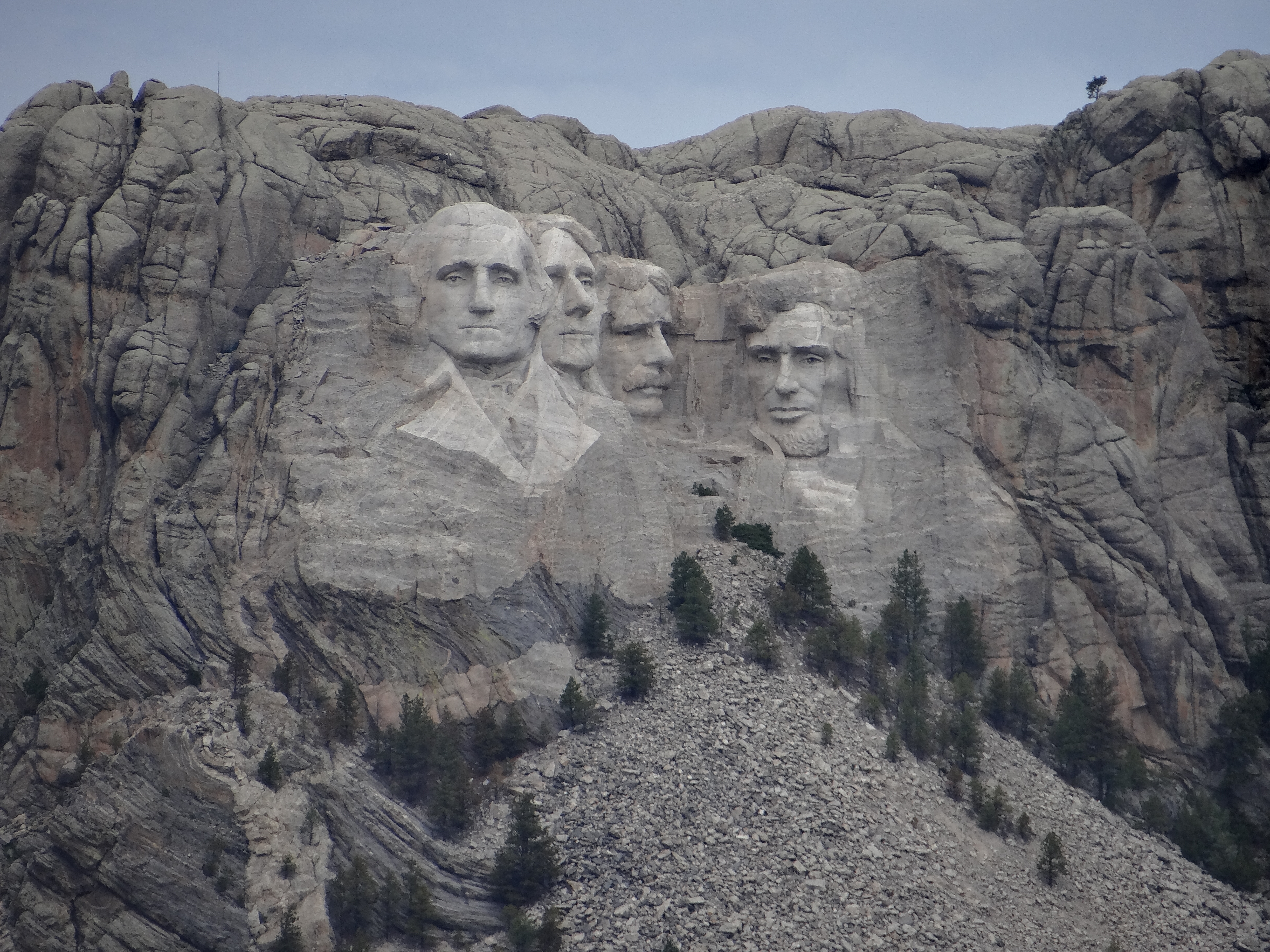
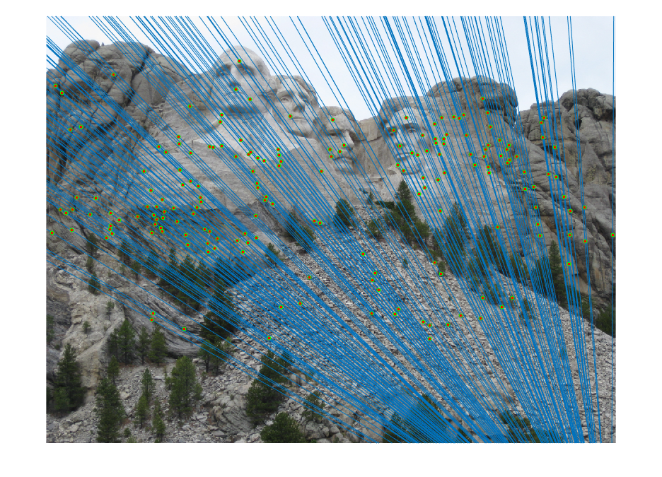
Mt. Rushmore
 |
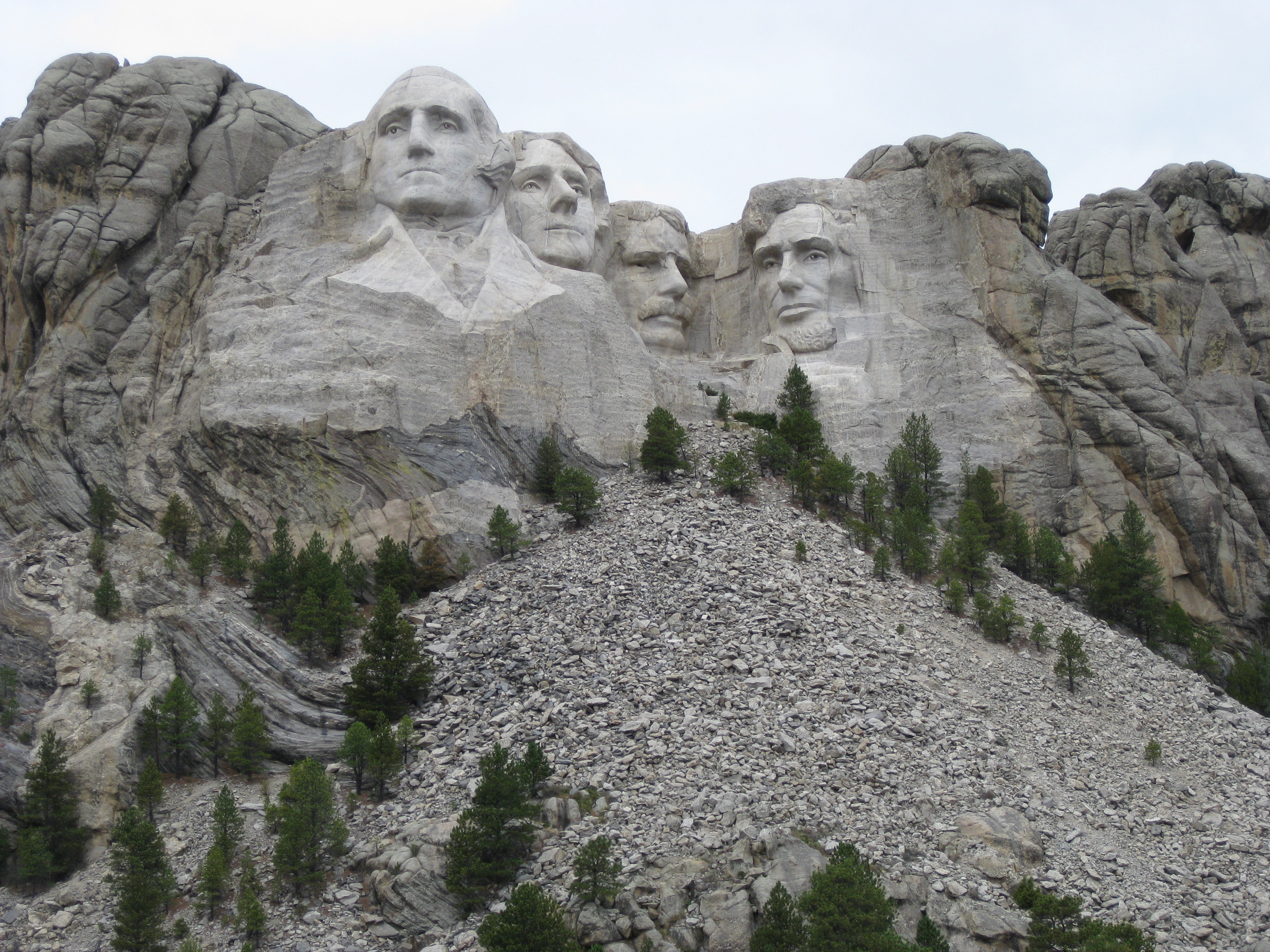 |
| fig. 5 Picture 1 original | fig. 6 Picture 2 original |
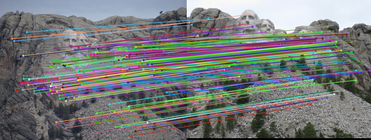 |
| fig. 7 Matching on inliers found from RANSAC |
 |
 |
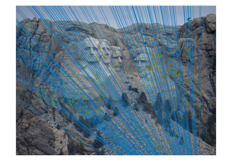
| fig. 8 Epipolar lines on picture 1 | fig. 9 Epipolar lines on picture 2 |
It is clear to see that almost all matches are correct, and the epipolar lines all fit through the points.
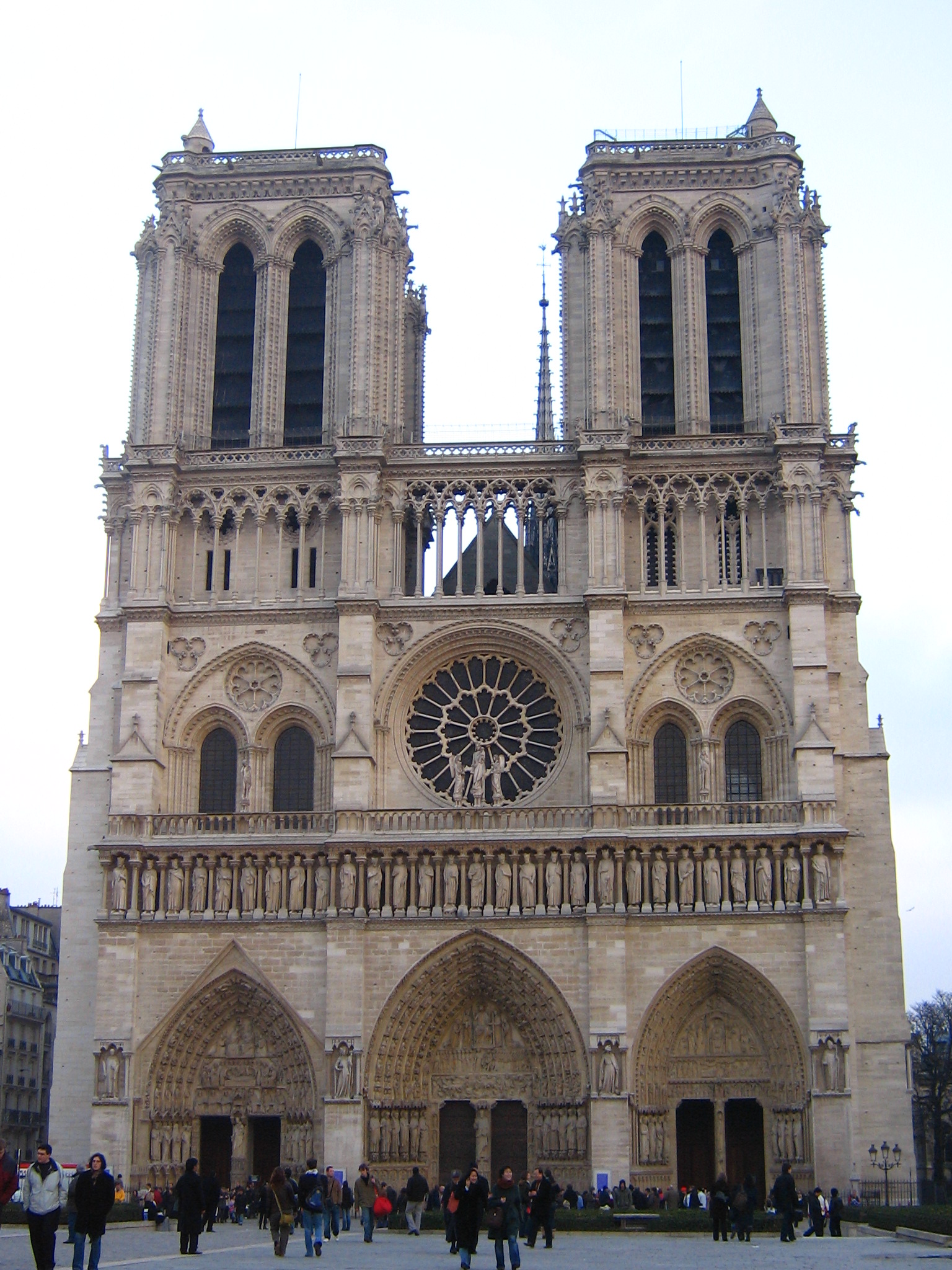
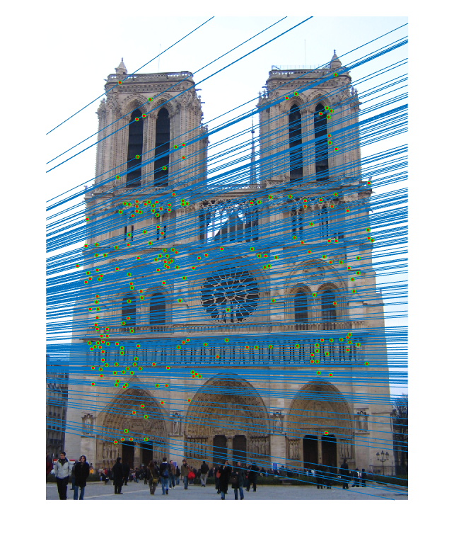
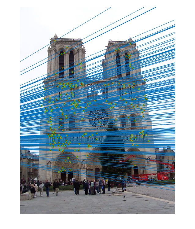
Notre Dame
 |
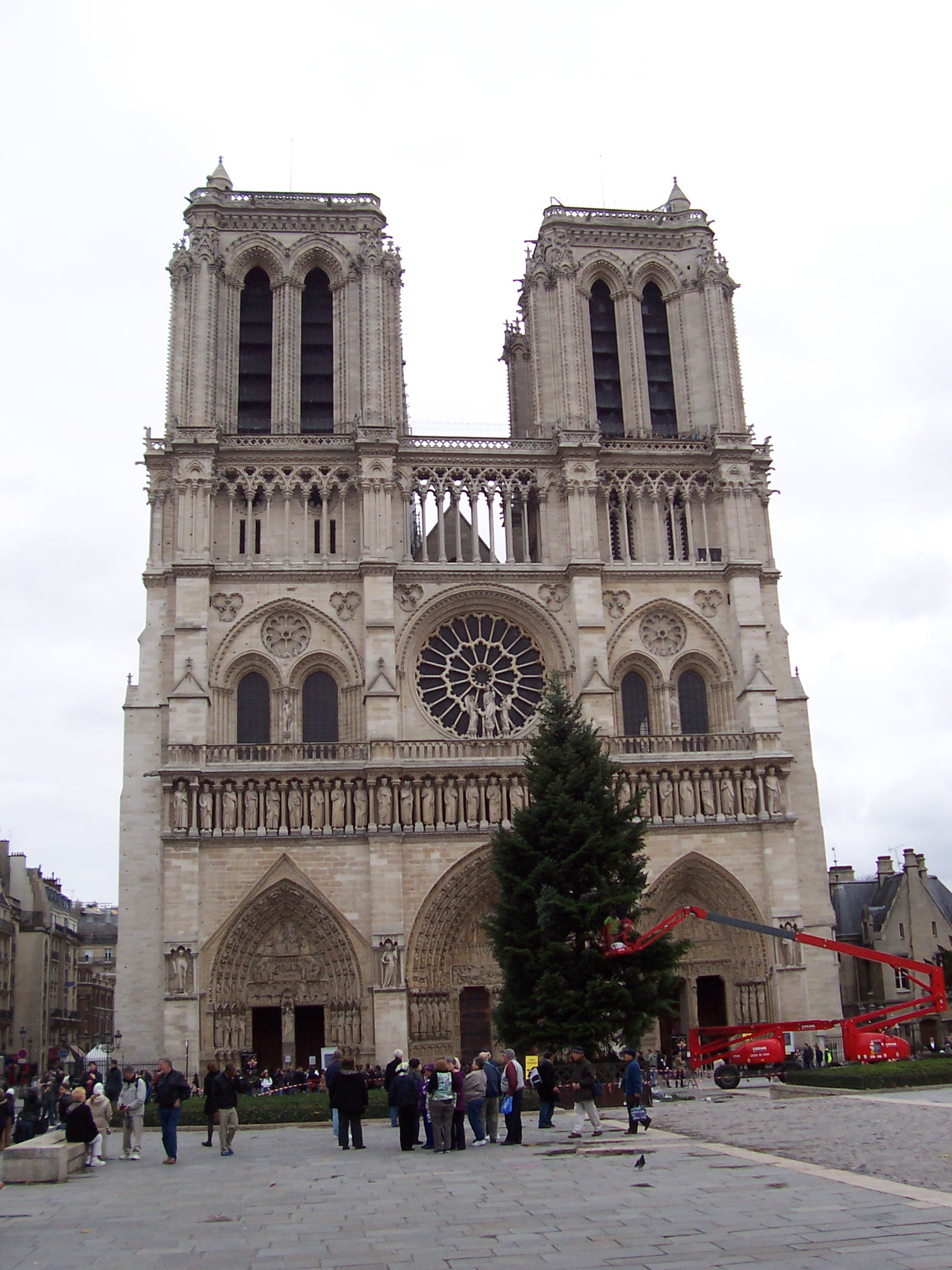 |
| fig. 10 Picture 1 original | fig. 11 Picture 2 original |
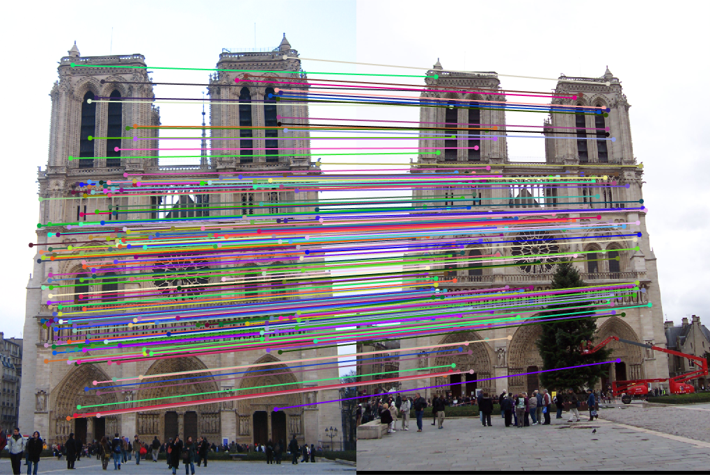 |
| fig. 12 Matching on inliers found from RANSAC |
 |
 |
| fig. 13 Epipolar lines on picture 1 | fig. 14 Epipolar lines on picture 2 |
Again, the matches seem to be of an extremely high accuracy, and the epipolar lines fit the points.
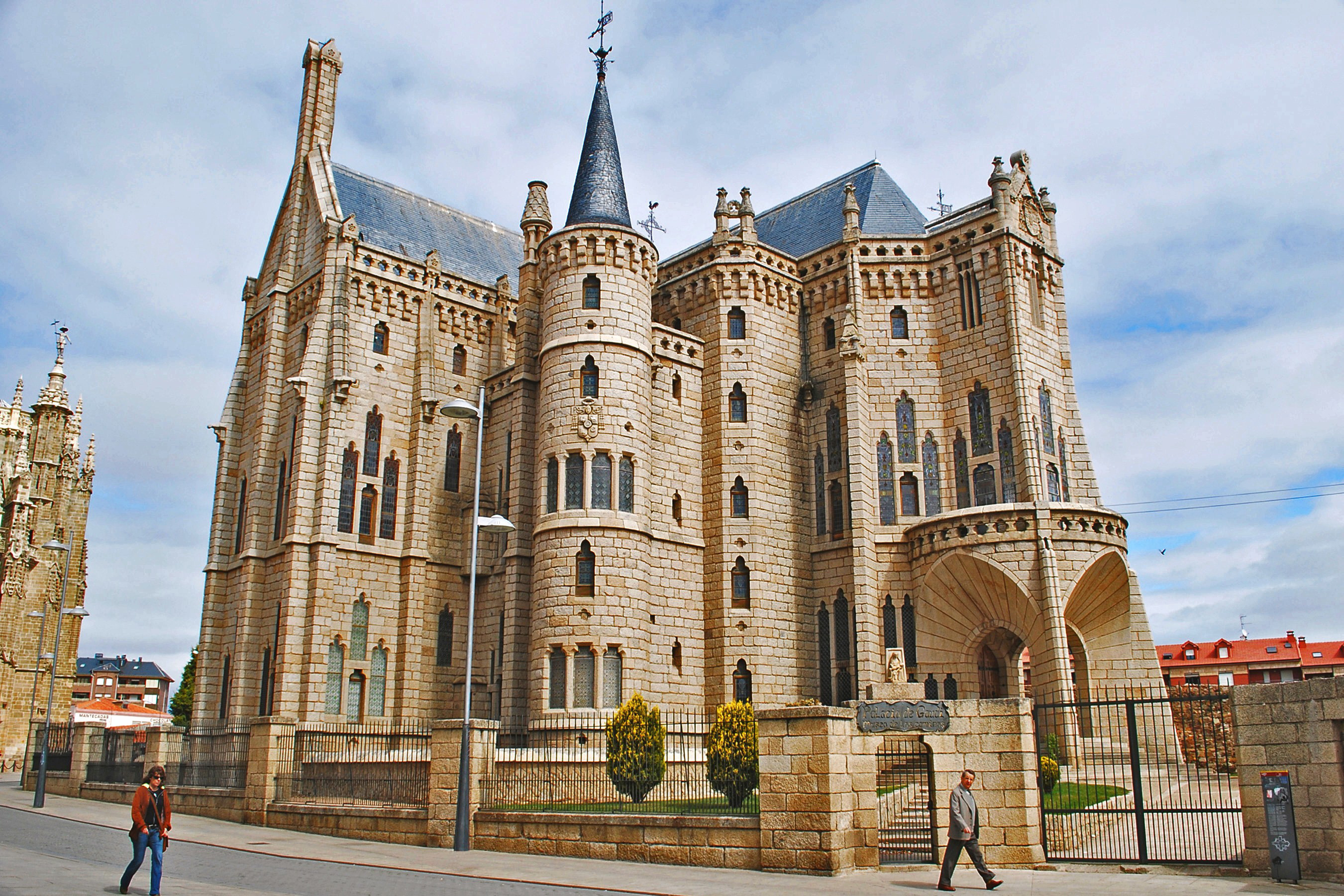
Episcopal Palace by Gaudí
 |
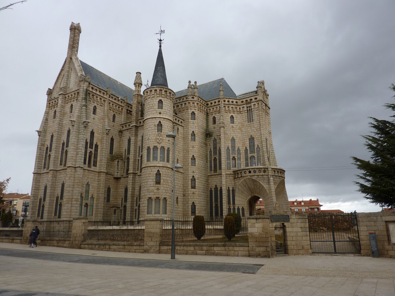 |
| fig. 15 Picture 1 original | fig. 16 Picture 2 original |
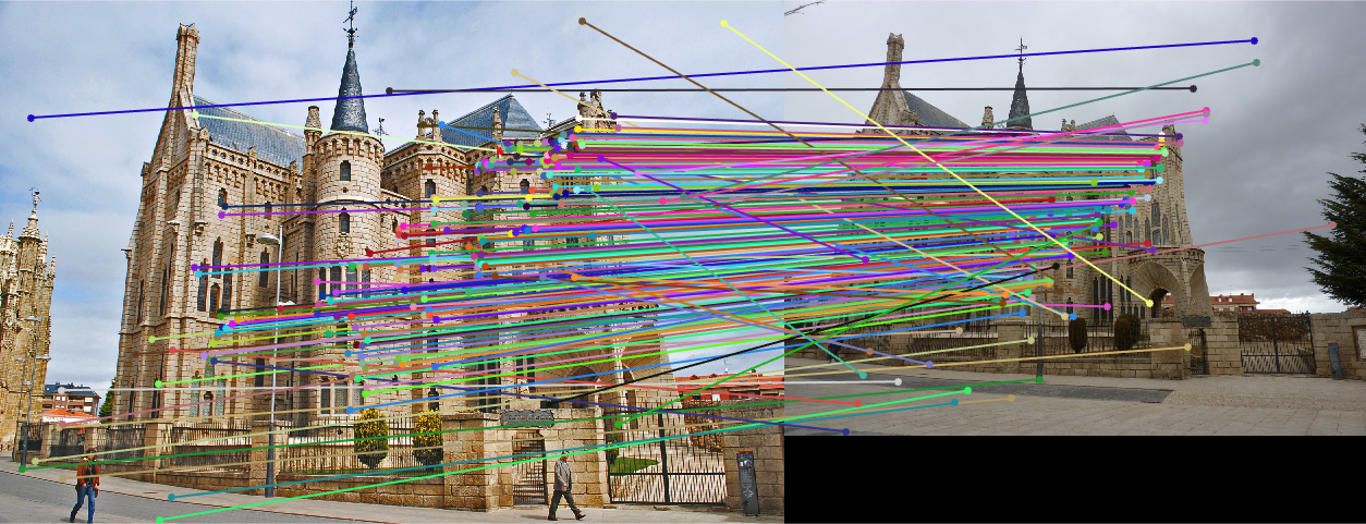 |
| fig. 17 Matching on inliers found from RANSAC |
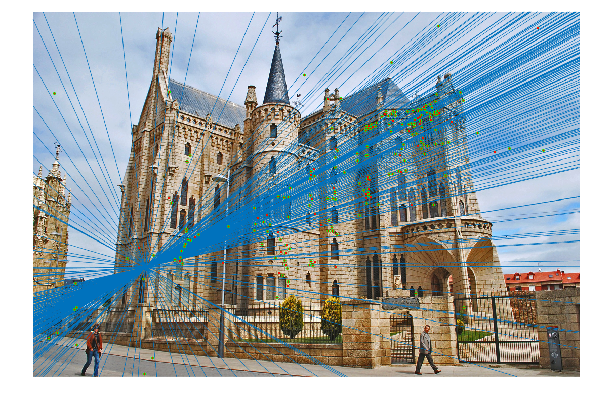 |
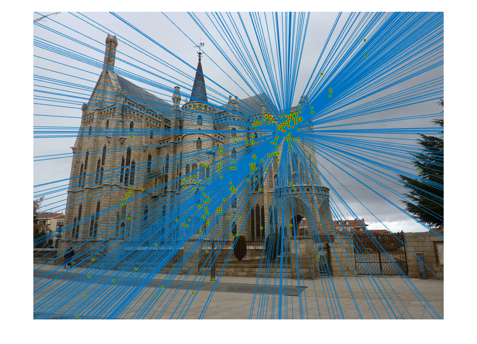 |
| fig. 18 Epipolar lines on picture 1 | fig. 19 Epipolar lines on picture 2 |
Much like in the last project involving the Episcopal Palace, good matches were few and far between. It also appears that the epipolar lines do not match most of the points, with a slight skew.
Addendum: Recalculating F with all Inliers
After all was said and done with RANSAC, it was possible to re-estimate the fundamental matrix with all inliers found, instead of the 9 randomly sampled. When this was done, very little changes were seen in the matches and epipolar lines. In face, for Mt. Rushmore, the matches were exactly the same. As such, I decided against including this recalculation in the final analysis: it did not appear to make a difference. It is unsure whether or not re-estimating the F matrix would aid in the matching, considering these inliers were found via another, simpler, similar F matrix.