Project 3
Camera Calibration and Fundamental Matrix Estimation with RANSAC
Part I: Camera Projection Matrix
We compute the camera projection matrix that goes from world 3D coordinates to 2D image coordinates by solving a system of linear equations with 11 unknown variables (M11, M12, M13, M14, M21, M22, M23, M24, M31, M32, M33). For each of the points in 3D (X1, Y1, Z1), we map it to a 2D points (u1, v1). We need at least 11 values to solve for the unknowns and as we have 2 values per 2D point, we only need 6 or more points.
Assume that the equation is of the form AM = b, and we need to find M.
                                                     [M11       [ u1
                                                      M12         v1
                                                      M13         .
                                                      M14         .
[ X1 Y1 Z1 1 0  0  0  0 -u1*X1 -u1*Y1 -u1*Z1          M21         .
  0  0  0  0 X1 Y1 Z1 1 -v1*X1 -v1*Y1 -v1*Z1          M22         .
  .  .  .  . .  .  .  .    .     .      .          *  M23   =     .
  Xn Yn Zn 1 0  0  0  0 -un*Xn -un*Yn -un*Zn          M24         .
  0  0  0  0 Xn Yn Zn 1 -vn*Xn -vn*Yn -vn*Zn ]        M31         .
                                                      M32         un
                                                      M33         vn ]
We solve using least squares with the '\' operator (M = A\b), reshape the matrix, multiply it with -0.5968 to obtain the expected Camera Projection Matrix as follows.
M_ = [ -0.4583  0.2947  0.0139 -0.0040
       0.0509  0.0546  0.5410  0.0524
      -0.1090 -0.1784  0.0443  -0.5968 ]
Once we have the camera projection matrix M, to find the camera center in world coordinates we find M = [Q | m4] as being made up of a 3x3 - Q and a 4th - m_4.
We now compute the center of the camera C = -Q' * m_4. (< -1.5125, -2.3515, 0.2826 >).
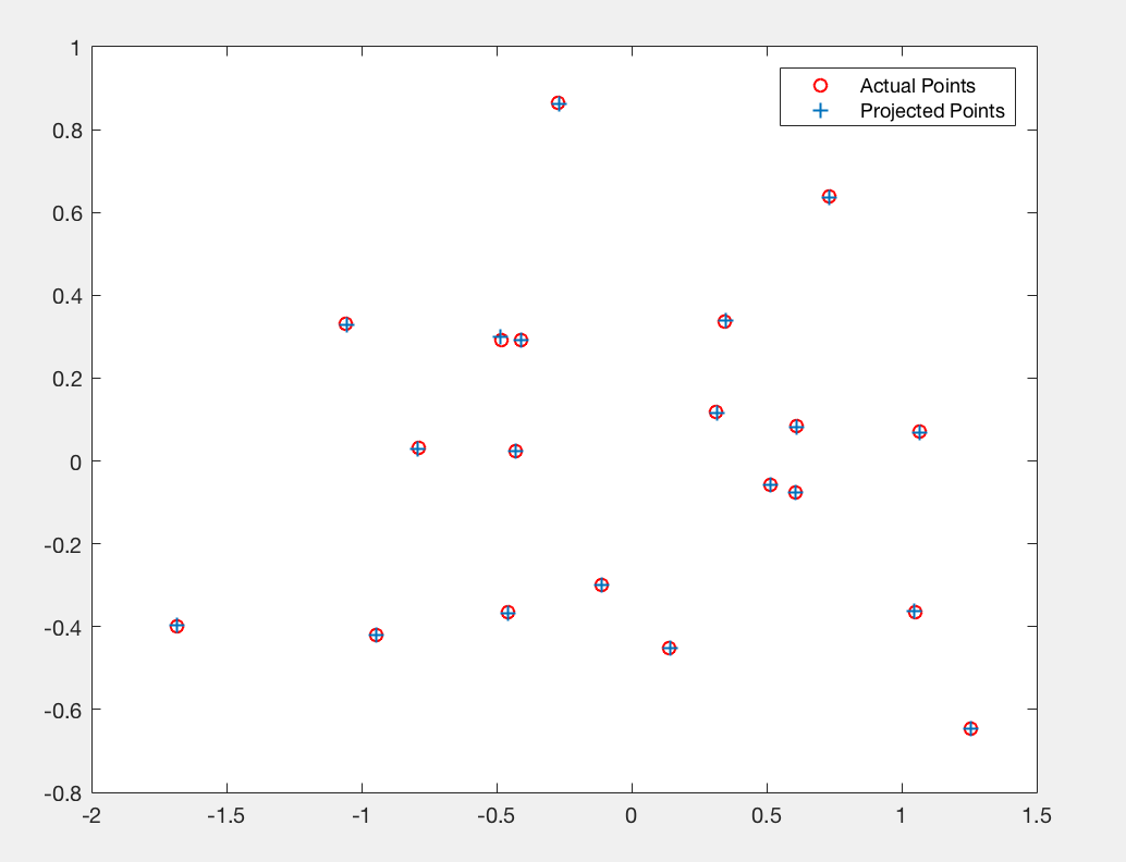
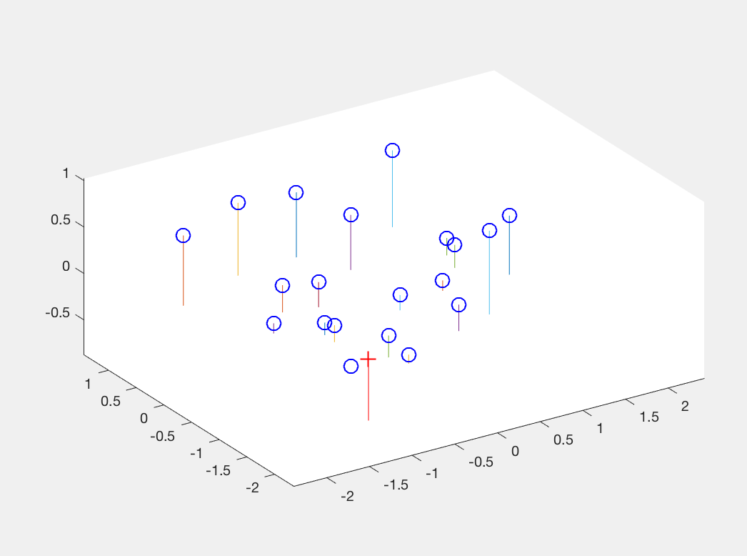
Output
| Expected vs Actual |
Camera View |
|
|
Part II: Fundamental Matrix Estimation
We estimate the mapping of points in one image to lines in another by means of the fundamental matrix. Given corresponding points we get one equation per point pair.
As the least squares estimate of F is full rank and that of the fundamental matrix is a rank 2 matrix, we must reduce its rank using singular value decomposition (USV' = F). We can then estimate a rank 2 matrix by setting the smallest singular value in S to zero (S_). The fundamental matrix is now calculated as F = US_V'.
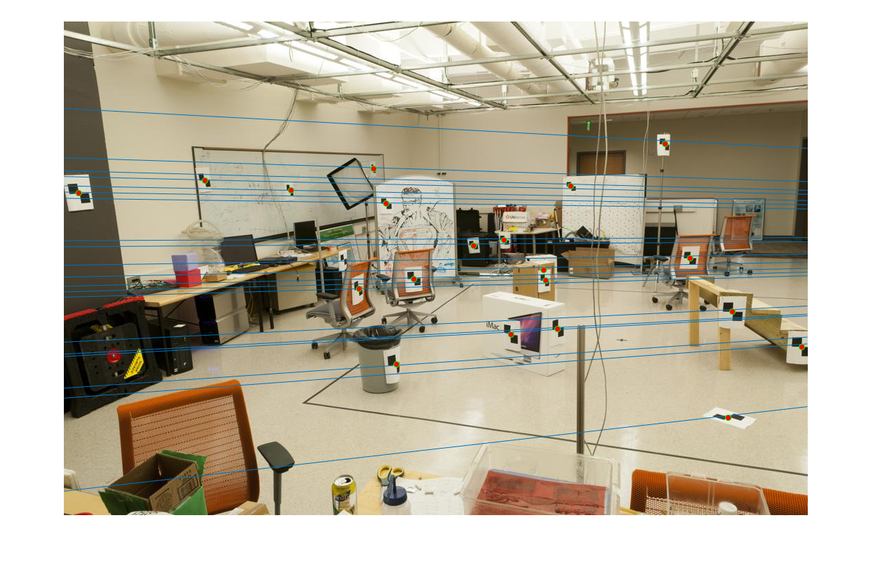
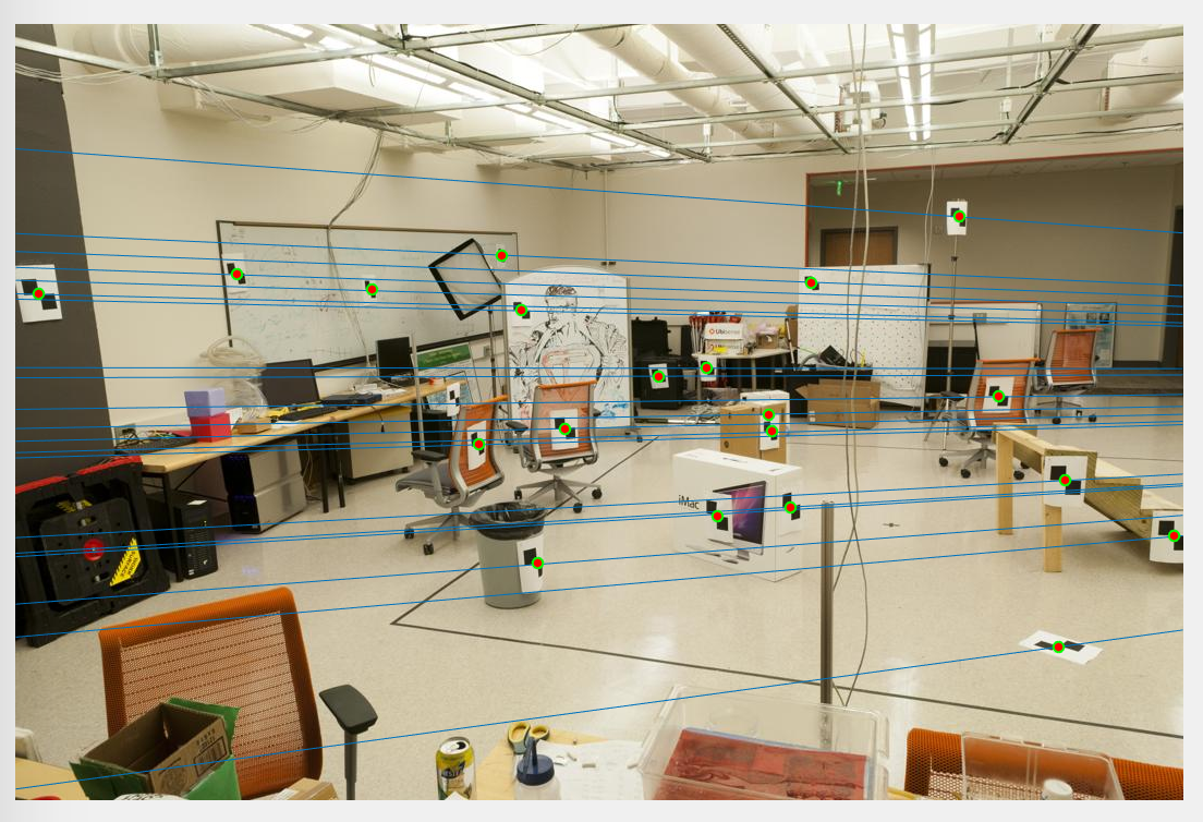
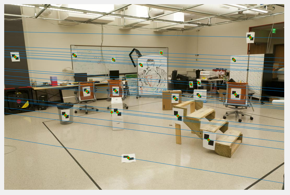
Extra Credit: Normalization
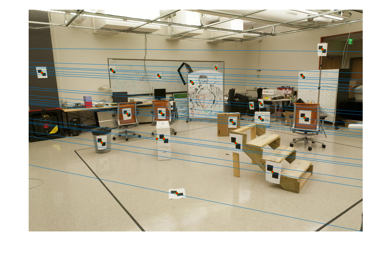
We normalize the points to mean 0 and standard deviation 1, and use these new points as the input for computing the fundamental matrix. The epipolar lines pass through the points more precisely with normalization. The difference in the output can be visualized below.
Without Normalization
With Normalization
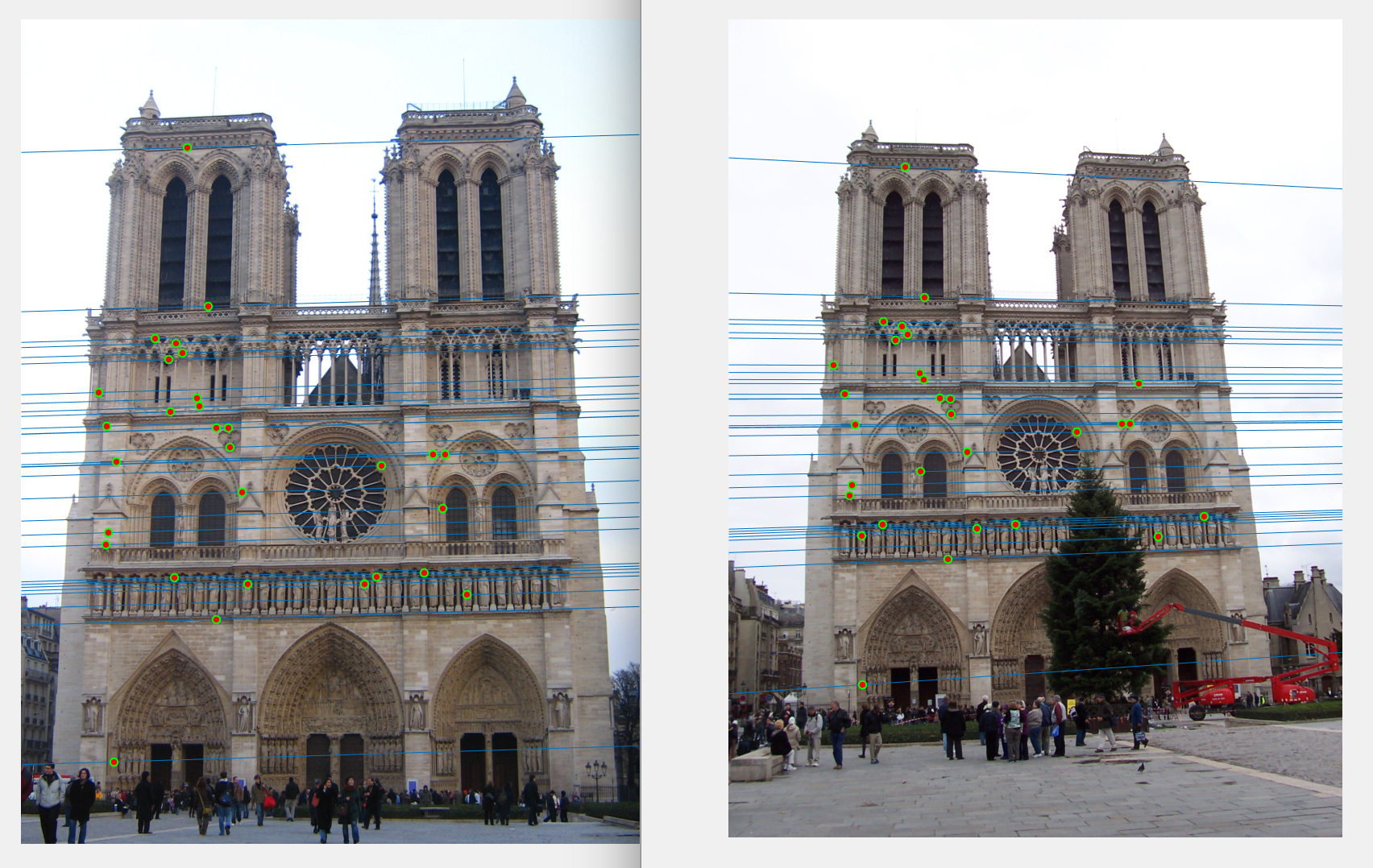
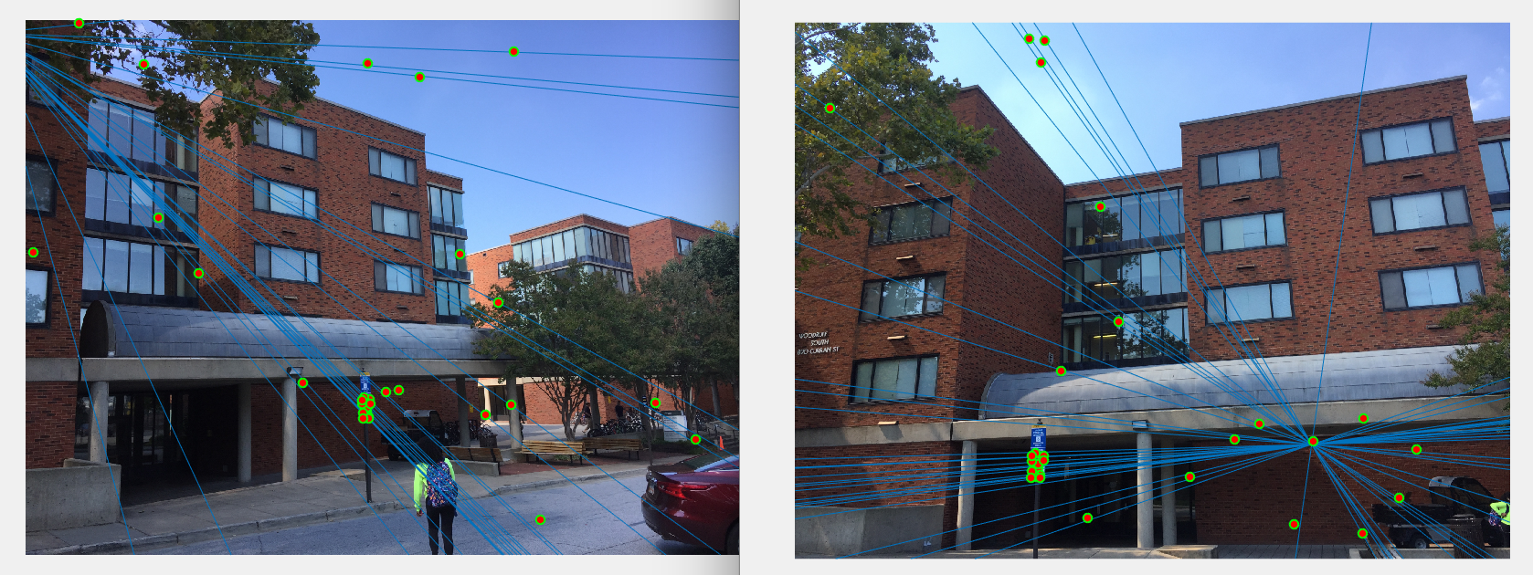
Part III: Fundamental Matrix with RANSAC
Using unreliable point correspondences computed with SIFT, using one to one point correspondence metrics will not give suitable solutions (eg : least squares regression) due to the presence of multiple outliers.
Instead we follow the following procedure (RANSAC) to calculate the "best" fundamental matrix.
Using 8 point correspondences we solve for the fundamental matrix using the function in part II, and then count the number of inliers. Inliers are point correspondences that fall within a certain threshold or "agree" with the estimated fundamental matrix.
RANSAC
- Sample 8 point correspondences from our dataset.
- Estimate the fundamental matrix using these points. Lets call it Fmatrix.
- Count the number of inliers (from the remaining dataset) and thresholding points if x'Fx > 0.1 (where x is a test ppint).
- Run the above steps for 2000 iterations and pick the model (fundamental matrix) with the maximum number of inliers
- Return the final best fundamental matrix and the best 30 points that fit this model.
Threshold (0.08)
| Type |
View 1 vs View 2 |
Best Correspondences |
| Notre Dame |
|
 |
| Mount Rushmore |
|
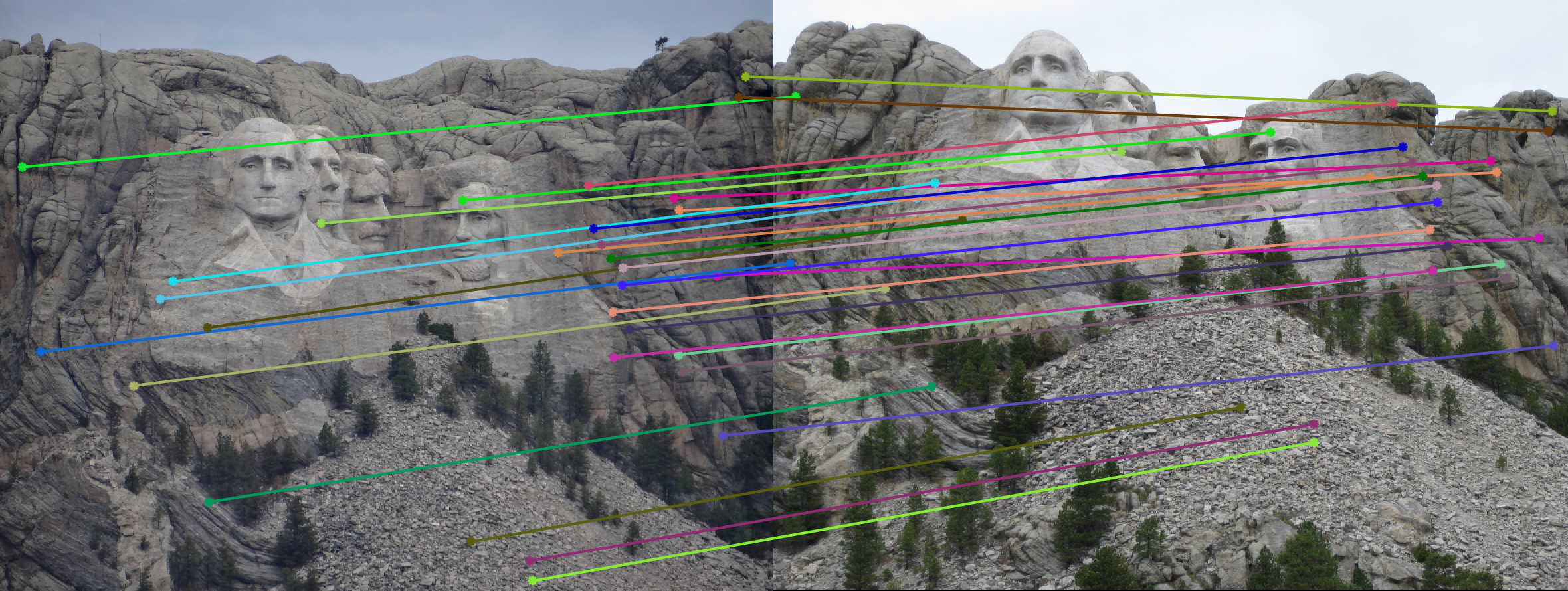 |
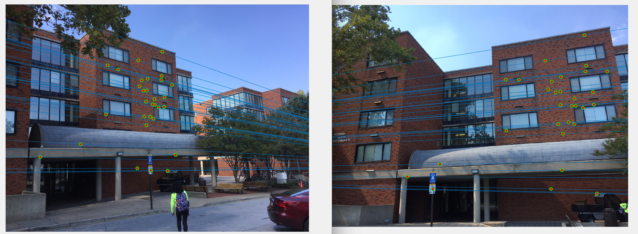
| Woodruff Dorm |
|
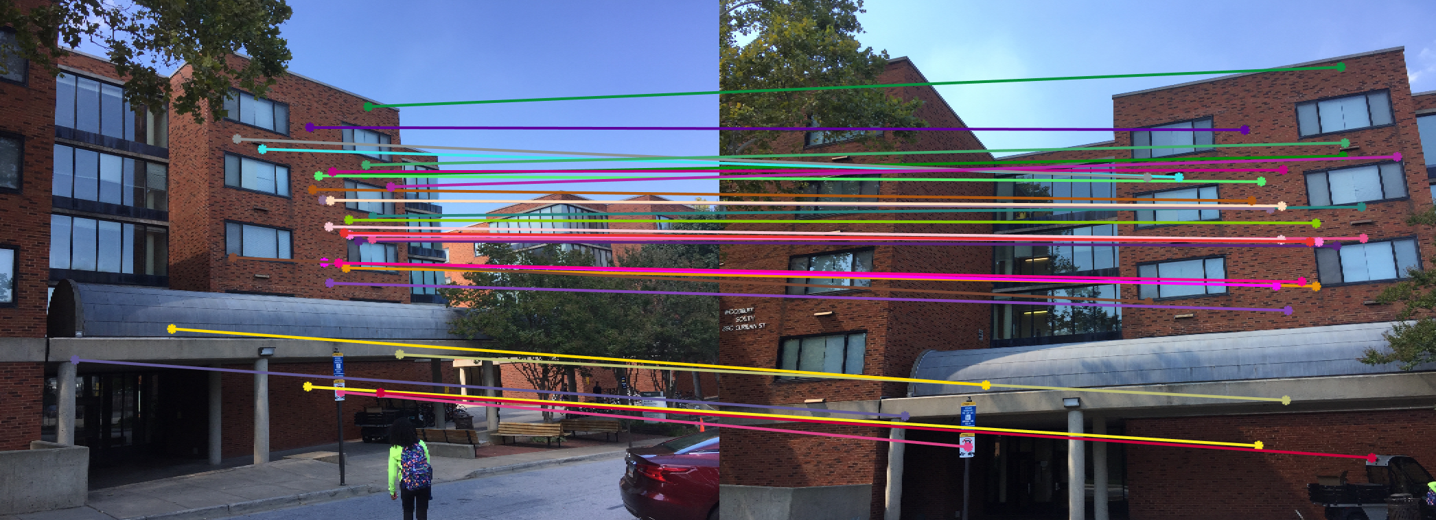 |
Erroneous results with a High Threshold (1.5)
| Type |
View 1 vs View 2 |
Best Correspondences |
| Woodruff Dorm |
|
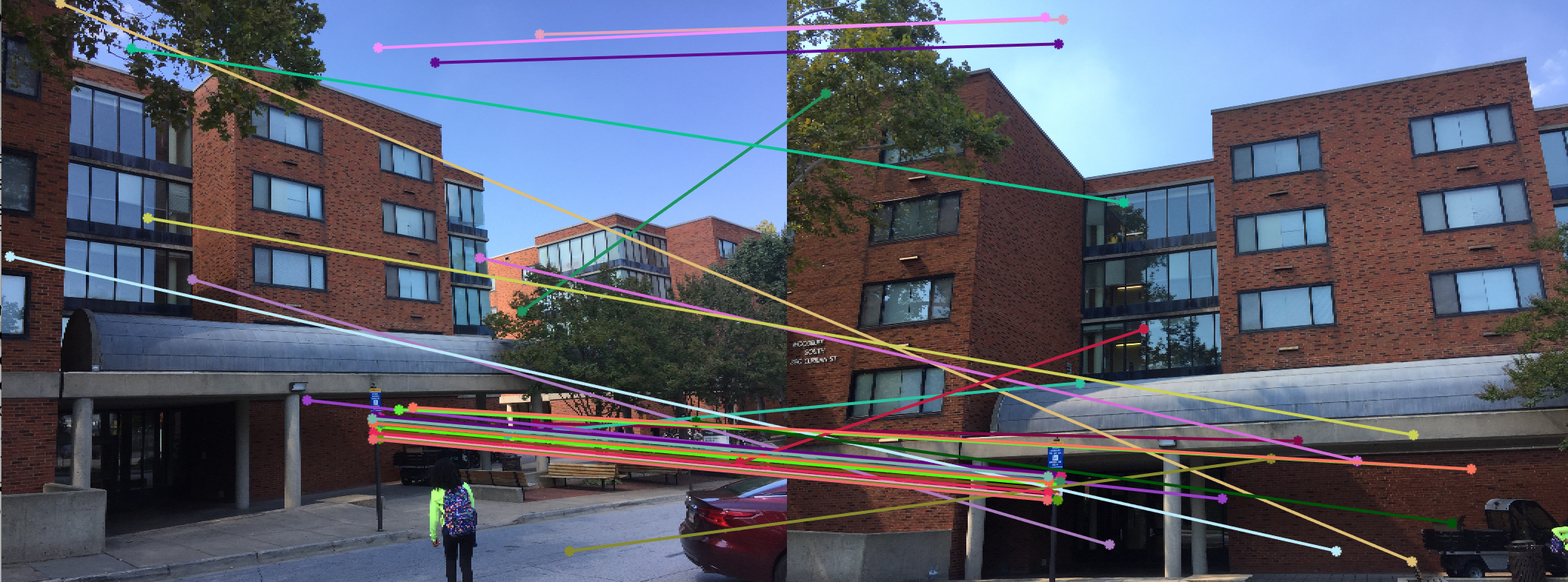 |