Project 3 / Camera Calibration and Fundamental Matrix Estimation with RANSAC
This report consists of 3 parts relating to analysis of
- Camera Projection Matrix Estimation
- Fundamental Matrix Estimation
- Fundamental Matrix Estimation with RANSAC
1. Camera Projection Matrix Estimation
Camera projection matrix estimation is performed by first setting up a homogenous system of equations. SVD is used on the homogenous equation system to find out the camera calibration matrix
Camera Projection Matrix Code
function M = calculate_projection_matrix( Points_2D, Points_3D )

homogenous_2D = [Points_2D ones(size(Points_2D,1),1)];
homogenous_3D = [Points_3D ones(size(Points_3D,1),1)];
A = [];
for row=1:size(Points_3D,1)
    point_3d = homogenous_3D(row,:);
    point_2d = homogenous_2D(row,:);
    zero_cols = zeros(1,size(point_3d,2));
    u_row = [point_3d zero_cols -point_2d(1,1)*point_3d];
    v_row = [zero_cols point_3d -point_2d(1,2)*point_3d];
    A = [A;u_row;v_row];
end
[U, S, V] = svd(A);
M = V(:,end);
M = reshape(M,[],3)';
end
Results
Projection matrix for normalized points
    0.4583   -0.2947   -0.0140    0.0040
   -0.0509   -0.0546   -0.5411   -0.0524
    0.1090    0.1783   -0.0443    0.5968
Camera center for normalized points
   -1.5127
   -2.3517
    0.2826

Projections

Camera
Projection matrix for optional points
0.0069   -0.0040   -0.0013   -0.8267
0.0015    0.0010   -0.0073   -0.5625
0.0000    0.0000   -0.0000   -0.0034
Camera center for optional points
	303.1000
  	307.1843
   	30.4217

Projections

Camera
2. Fundamental Matrix Estimation
Fundamental Matrix estimation is being done by setting up homogenous system of equations. Normalization has been implemented as part of extra credit. Normalization has been done using standard deviation and linear transformation as provided in the assignment description. Although normalization does not impact the output in part 2, the analysis of normalization has been detailed out in later parts of the report.
Fundamental Matrix Estimation Code
function [ F_matrix ] = estimate_fundamental_matrix(Points_a,Points_b)

homogenous_a = [Points_a ones(size(Points_a,1),1)];
homogenous_b = [Points_b ones(size(Points_b,1),1)];

%normalization
c_uv = mean(Points_a);
s = std(Points_a);
s_matrix = [[s(1,1) 0 0];[0 s(1,2) 0];[0 0 1]];
c_matrix = [[1 0 -c_uv(1,1)]; [0 1 -c_uv(1,2)]; [0 0 1]];
T_a = s_matrix * c_matrix;

for point=1:size(homogenous_a,1)
    homogenous_a(point,:) = T_a * transpose(homogenous_a(point,:));
end

c_uv = mean(Points_b);
s = std(Points_b);
s_matrix = [[s(1,1) 0 0];[0 s(1,2) 0];[0 0 1]];
c_matrix = [[1 0 -c_uv(1,1)]; [0 1 -c_uv(1,2)]; [0 0 1]];
T_b = s_matrix * c_matrix;

for point=1:size(homogenous_b,1)
    homogenous_b(point,:) = T_a * transpose(homogenous_b(point,:));
end

%Build the matrix for equations
equation_matrix = [];
for row=1:size(homogenous_a,1)
    point_a = homogenous_a(row,:);
    point_b = homogenous_b(row,:);
    combined_row = [point_b .* point_a(1,1), point_b .* point_a(1,2), point_b .* point_a(1,3)];
    equation_matrix = [equation_matrix;combined_row];
end

[U, S, V] = svd(equation_matrix);
F = V(:,end);
F = reshape(F,[3 3])';
F = transpose(F); % visualization code assumed transpose version of the matrix compared to lecture slides

%Fix the rank
[U, S, V] = svd(F);
S(3,3) = 0;
F_matrix = U * S * transpose(V);
F_matrix = transpose(T_b) * F_matrix * T_a;
end
Results
Estimate of Fundamental Matrix
	F_matrix =

   -0.0000    0.0000   -0.0045
    0.0000   -0.0000    0.0292
    0.0001   -0.0467    1.9942
Image results

|
|
3. Fundamental Matrix Estimation with RANSAC
RANSAC code
RANSAC has been used to estimate the best possible fundamental matrix given correspondences containing both good and bad matches. RANSAC for most observations given in this report has been run for 5000-8000 iterations depending on the number of possible matching points given by VLSeat. RANSAC helps in rejecting outliers that were otherwise identified as matches. This is done by estimating a fundamental matrix for a random sample of minimum number of points - 8, finding out how many inliers agree with this fundamental matrix and how many outliers disagree with this matrix. The error is computed using the fundamental property of epipolar geometry where a point in one image has to be on the corresponding epipolar line in the other image. Any deviation from 0 given the linear product combination is thresholded to differentiate between outliers and inliers. The best fundamental matrix is reported once all iterations have completed.
function [ Best_Fmatrix, inliers_a, inliers_b] = ransac_fundamental_matrix(matches_a, matches_b)


max_inliers = 0;
inliers_a = [];
inliers_b = [];
inliers = [];

for N=1:7000
    random_indices = randperm(size(matches_a,1),8);
    sampled_points_a = matches_a(random_indices,:);
    sampled_points_b = matches_b(random_indices,:);
    f_matrix = estimate_fundamental_matrix(sampled_points_a, sampled_points_b);
    curr_inliers = 0;
    curr_inliers_a = [];
    curr_inliers_b = [];
%     curr_inliers_with_err = [];
    for point = 1:size(matches_a,1)
        error = [matches_b(point,:) 1] * f_matrix * transpose([matches_a(point,:) 1]);
        if abs(error) < 0.05
            curr_inliers = curr_inliers + 1;
            curr_inliers_a = [curr_inliers_a;matches_a(point,:)];
            curr_inliers_b = [curr_inliers_b;matches_b(point,:)];
%             curr_inliers_with_err = [curr_inliers_with_err; [matches_a(point,:) matches_b(point,:) abs(error)]];
        end
    end
    if curr_inliers > max_inliers
        Best_Fmatrix = f_matrix;
        inliers_a = curr_inliers_a;
        inliers_b = curr_inliers_b;
%         inliers = curr_inliers_with_err;
        max_inliers = curr_inliers;
    end
end
% [d1,d2] = sort(inliers(:,5));
% inliers = inliers(d2,:);
% inliers_a = inliers(1:30,1:2);
% inliers_b = inliers(1:30,3:4);

% random_indices = randperm(size(inliers_a,1),min(30, size(inliers_a,1)));
% inliers_a = inliers_a(random_indices,:);
% inliers_b = inliers_b(random_indices,:);
end
Results
Correspondences Rushmore

Epipolar geometry

|

|
Observations
RANSAC has managed to remove most outliers except for a meagre number of outliers.
Above correspondences and epipolar was constructed using 5000 iterations, 8 point fundamental matrix estimation, 0.005 threshold value for absolute error. It resulted in 151 correspondences
Observations with normalized points
Even for a simple image like Mount Rushmore, normalization of points before estimating fundamental matrix yields better correspondences and epipolar geometry. Images are given below.
In case of Episcopal Gaudi, normalization seems to improve the correspondences a lot better than any other image pair. Normalization also seems to balance the bias towards certain co-ordinates as in the case of Mount Rushmore
Correspondences Rushmore with normalization
|
|

|
Left : Raw co-ordinates, Right : With normalized co-ordinates
Epipolar geometry with normalization

|
Epipolar geometry for other images
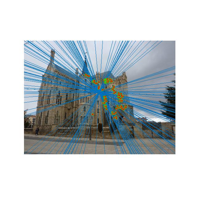
Gaudi without normalization

Gaudi without normalization
Bad Correspondences

|

|
Bad Epipolar geometry
Gaudi with normalization

Correspondences
|

|
Epipolar geometry
Notre Dame without normalization

Correspondences

|

|
Epipolar geometry