Project 3 / Camera Calibration and Fundamental Matrix Estimation with RANSAC
In this project our task was to learn about camera and scene geometry by completing three tasks:
- Find a Camera Projection Matrix that goes from world 3D coordinates to 2D image coordinates using corresponding points. Also find the camera center C.
- Estimate the Fundamental Matrix F given corresponding points between images by using linear regression.
- Estimate the Fundamental Matrix for realistic image pairs using RANSAC
- Do second and third task with normalized points which improve linear estimation of F
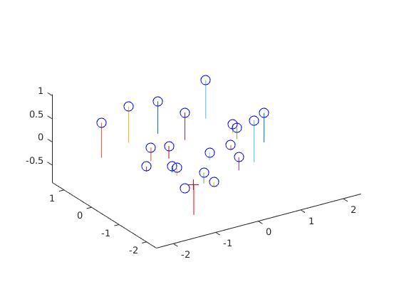
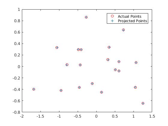
Part I: Camera Projection Matrix
In this part we compute the projection matrix by solving a linear system using corresponding world 3D points and image 2D points. In order to do this we setup a homogeneous set of equations in matrix form using the corresponding points and perform a linear regression on this set which is pretty straightforward. We obtain the following results and we obtain the correct M matrix after scaling and also the correct camera center:

Part II: Fundamental Matrix Estimation
Here we estimate the Fundamental Matrix given corresponding points between two ideal images by using linear regression. We follow the same path as before, building a linear system in matrix form using the corresponding points between images and then using singular value decomposition to solve the system. We obtain an F matrix which is rank 3, but the F matrix should be rank 2. We perform SVD on the matrix, change the third eigenvalue of the eigenvalue matrix to zero and then reconstruct the F matrix which now has rank 2. As you can see the results are good but some epipolar lines do not pass exactly through the points. This is fixed after performing the normalization of points which is the graduate credit portion of the project.
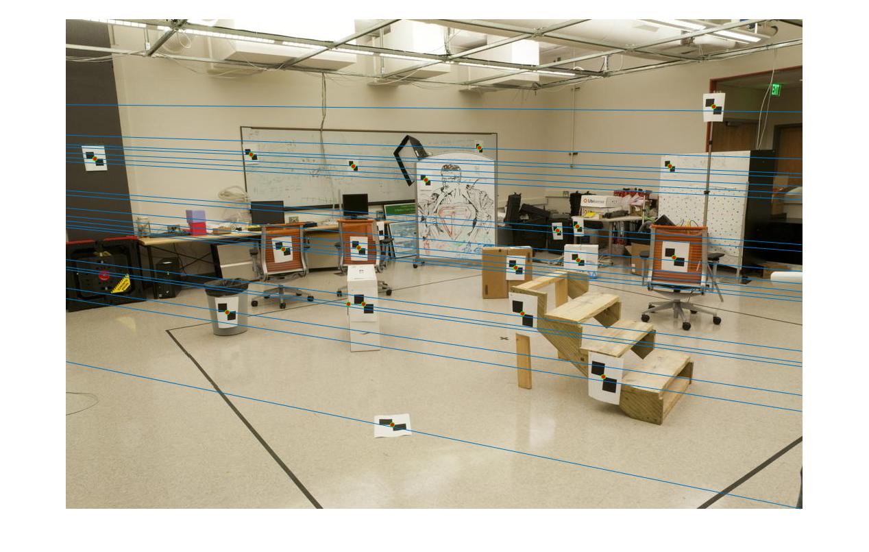
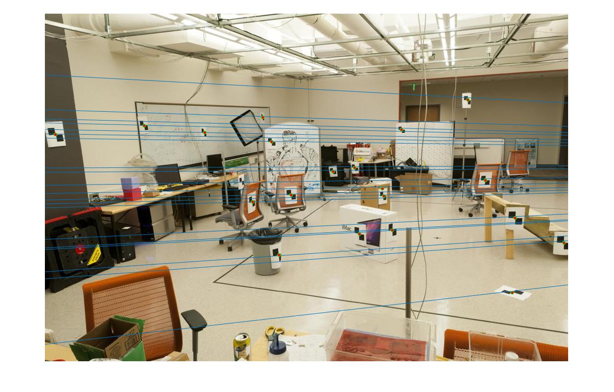
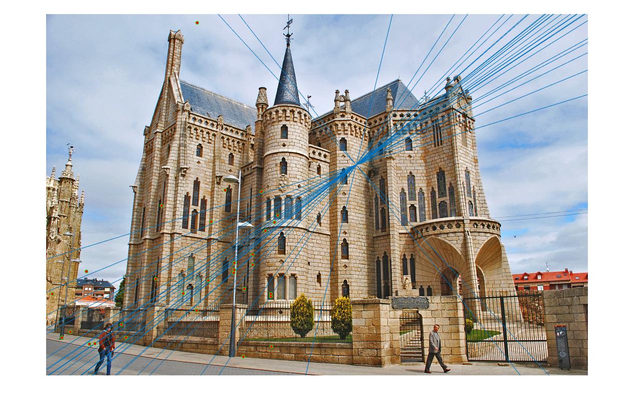
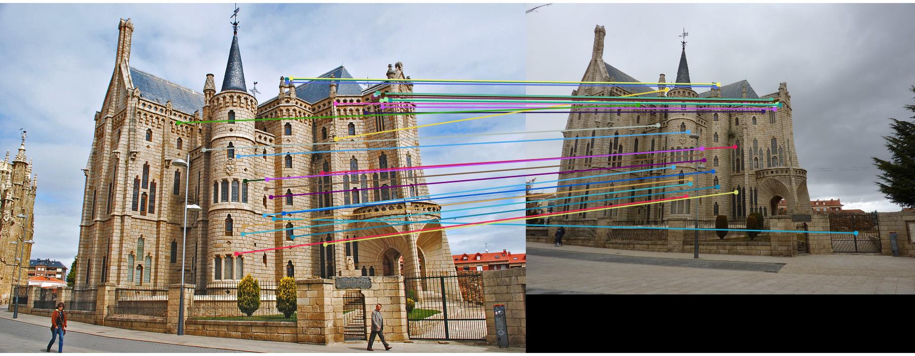
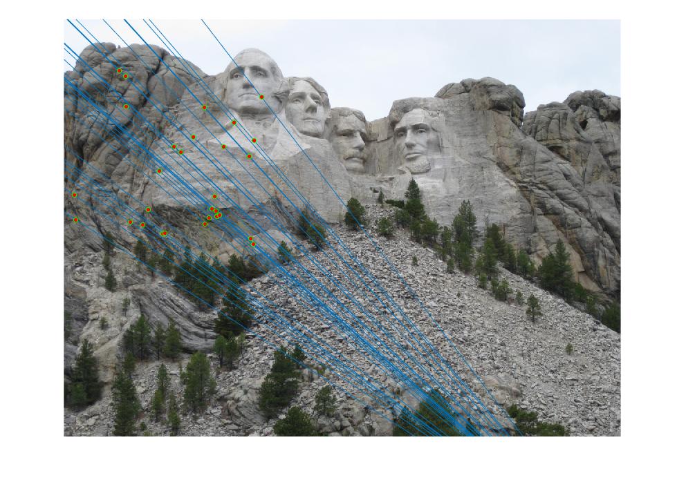
Part III: Fundamental Matrix with RANSAC
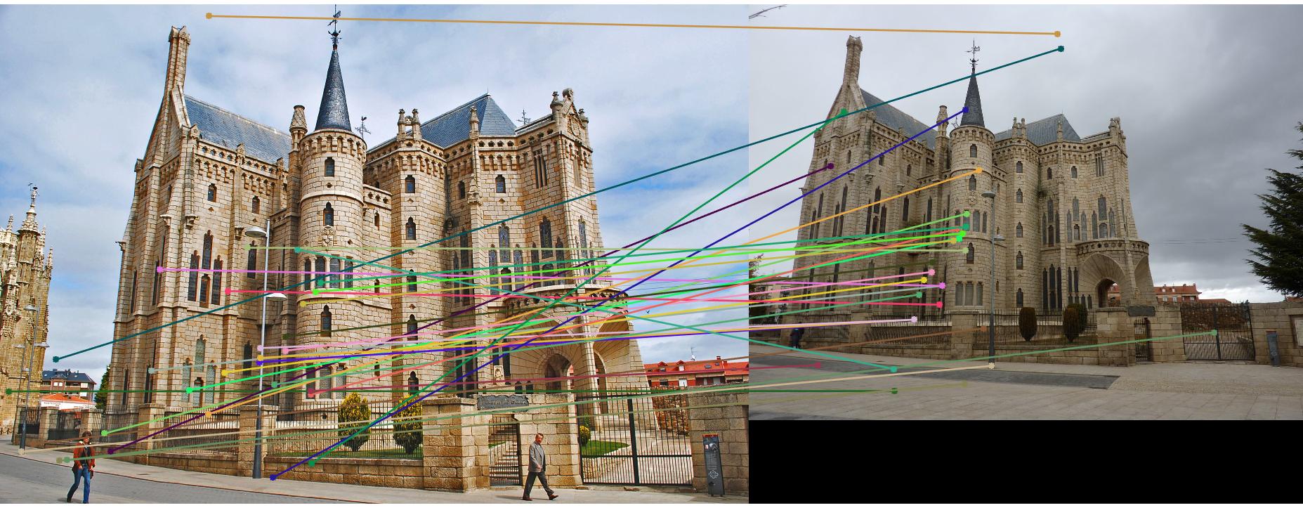
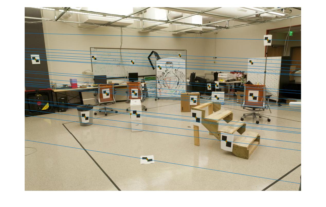
For two photographs of a scene it's hard to find perfect point correspondence which can then be used to regress a Fundamental Matrix. What we do is use SIFT matching to find point correspondences which will then be used to perform RANSAC and find an F matrix. For each iteration of RANSAC we pick 8 points and estimate the Fundamental Matrix using the code from Part II. For each point correspondence (x, x') we compute: 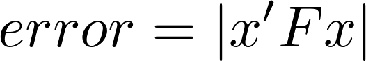
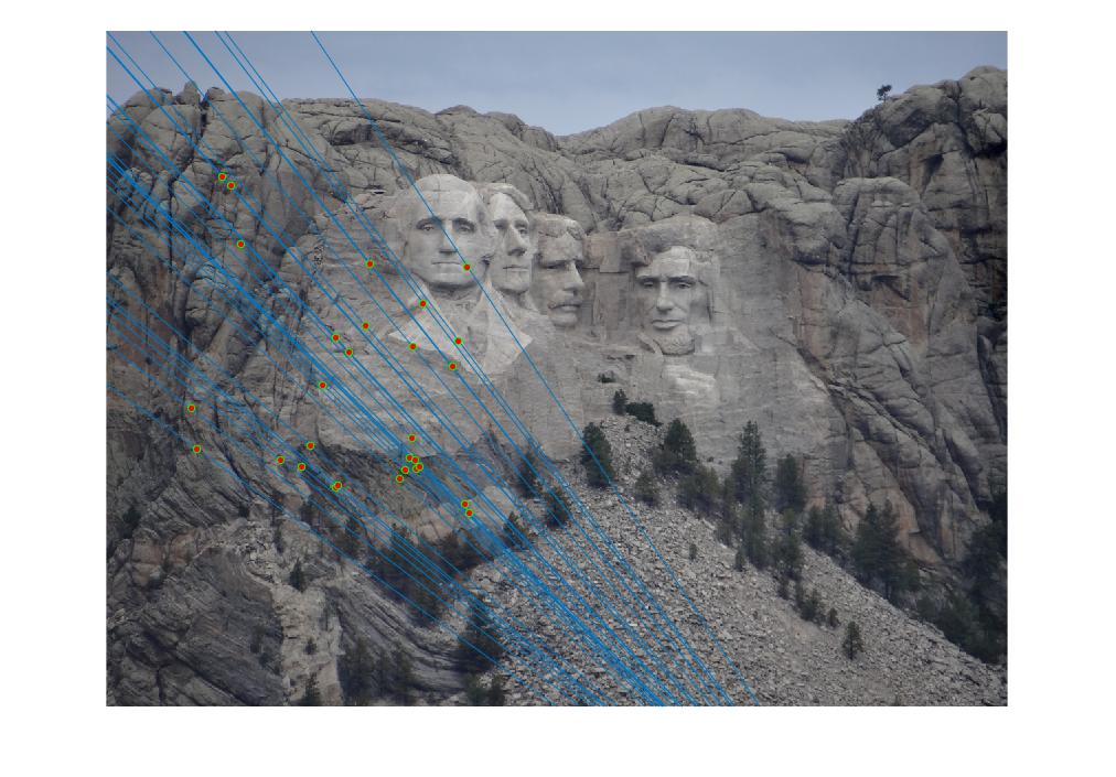
If the error is less than our set threshold then the points are inliers. We perform multiple iterations and we select the matrix that has the most inliers.
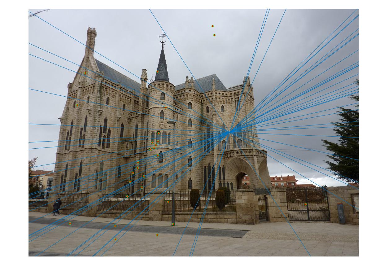
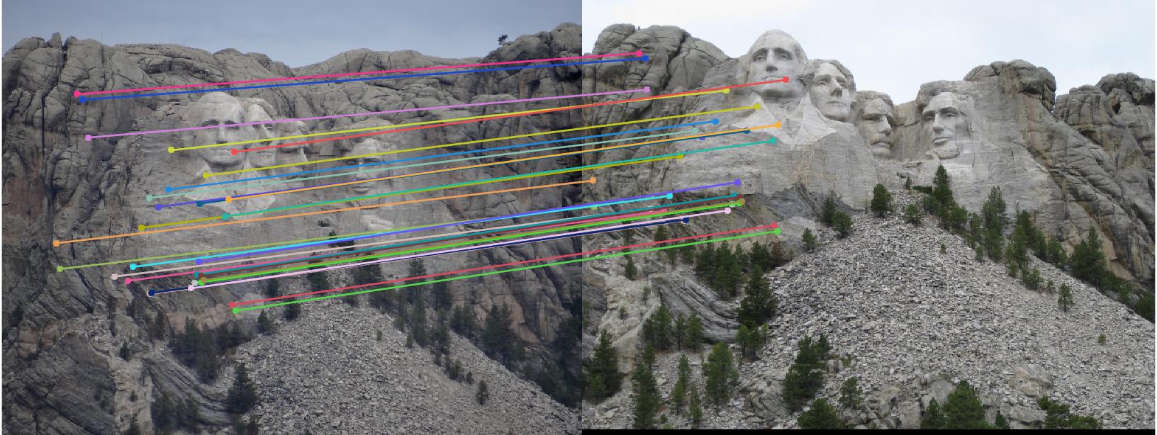
We spent a little bit of time tuning the threshold parameter before we implemented the extra credit. We proceeded by a sort of qualitative binary search in which we initialized the threshold to 1 and 0.0001, checked the qualitative results such as plot of matches and epipoles and the quantitative results such as number of inliers. We want to find a threshold that has the most inliers possible while still rejecting spurious matches. We used 3000 iterations for this test and 30 final matches. We found the best threshold to be between 0.1 and 0.2, and we stuck with 0.1 throughout the rest of the project. We then increased the number of iterations to 9000 to find better matrices. These are some results after having applied the extra credit. We will compare a cases of pre-extra credit and post-extra credit in the next section.
Extra Credit: Normalizing point coordinates.
As seen in class, to improve the estimation of the Fundamental Matrix we can decide to normalize the point coordinates before computing the linear regression. We do this by multiplying the homogeneous coordinates of our points by the Transformation matrix which is the product of the Scale and the Offset matrices as seen below.
c_u and c_v are the means of the u and v point coordinates. We have a choice for s, we could use the maximum coordinate of the points after subtracting the mean, or the standard deviation after substracting the mean, we could use two different s: one for the standard deviation of the first coordinate and the second coordinate. We found that all of these choices were good and almost equivalent. Below a comparison of the epipolar lines of part 2 before normalization, after normalization with s using max and after normalization with s using the standard deviation. We can see almost no difference between the last two, but the epipolar lines are much better than the non-normalized case. Note that the F matrix has to also be transformed and we do so by left-multiplying it by the transpose of T_b and right multiplying it by T_a after it has been reduced in rank.

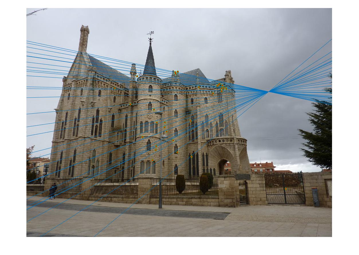
We ended up using the standard deviation method. Next we present before and after extra credit results for the gaudi image which are very much improved.