CS6476: Assignment 3

Paul Glotfelter

October 11, 2016

1 Introduction

This report summarizes the results and work for the third assignment for CS6476. This particular assignment dealt with estimating the camera center and fundamental matrix for image pairs and utilizing the estimate fundamental matrix for feature matching.

2 Part One

In this portion of the project, we handle the computation of the projection matrix, which projects 3-D world coordinates onto the 2-D image plane, and the camera center, which shows where the camera is located.

2.1 Determining the Projection Matrix

Given two images of the same scene, the projection matrix may be determined through a linear least squares algorithm, provided enough potentially corresponding points. As such, the projection matrix is given by

⌊ ⌋ ⌊ ⌋ X ⌈su ⌉ ||Y || sv = M ⌈Z ⌉, s 1

(1)

where M is the projection matrix from world into image coordinates and s is the scale. For this problem, we would like to fix s = 1. This result may be obtained via a few methods. In this case, we elected to use a Singular Value Decomposition (SVD) to obtain the desired, normalized solution.

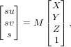
To solve for M one may re-write the problem as a linear system of equations as

[ ] Xi Yi Zi 1 0 0 0 0 − uiXi − uiYi − uiZi − ui M = 0. 0 0 0 0 Xi Yi Zi 1 − viXi − viYi − viZi − vi

(2)

In this case, we have elected to use an SVD to solve for M, resolving the scaling issue. Using this solution with the provided points yielded the matrix

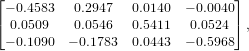⌊ ⌋ − 0.4583 0.2947 0.0140 − 0.0040 ⌈ 0.0509 0.0546 0.5411 0.0524 ⌉, − 0.1090 − 0.1783 0.0443 − 0.5968

(3)

where the residual was 0.0445.

2.2 Finding the Camera Center

Next, we compute the center of the camera utilizing M through the equation

C = − Q −1m4,

(4)

where M = [Q | m4 ] and Q ∈ ℝ³. Given the previously determined matrix M, we calculated the camera center to be

C = [− 1.5127 − 2.3517 0.2826]T

(5)

, which is very close to the supplied value in the assignment description. Fig 1 shows the relationship between the projected points, using M, and the actual points. Utilizing the non-normalized coordindates, the results closely resembled those of Fig. 1.

Figure 1: Displays the projected points versus the actual points via the projection matrix M from world to camera coordinates.

3 Part Two

This section contains work for estimating the fundamental matrix of the system. This matrix generates epipolar lines that relate two view of the same image. In particular, they allow one to determine where corresponding points lie in some line of the corresponding image, yielding a useful tool in a feature-matching pipeline.

3.1 Estimating the Fundamental Matrix

Given two images of the same scene, the fundamental matrix F between two scenes is such that

x′F x = 0,

(6)

where x′,x are from two corresponding images. Given 8 points from the images, it is possible to compute F. Again, we solve for F utilizing a system of linear equations in the form

[ ] A = xix′i yix′i x′i xiyi′ yiy′i y′i xi yi 1

(7)

Here, we utilize an SVD to solve the linear system of equations

AF = 0,

(8)

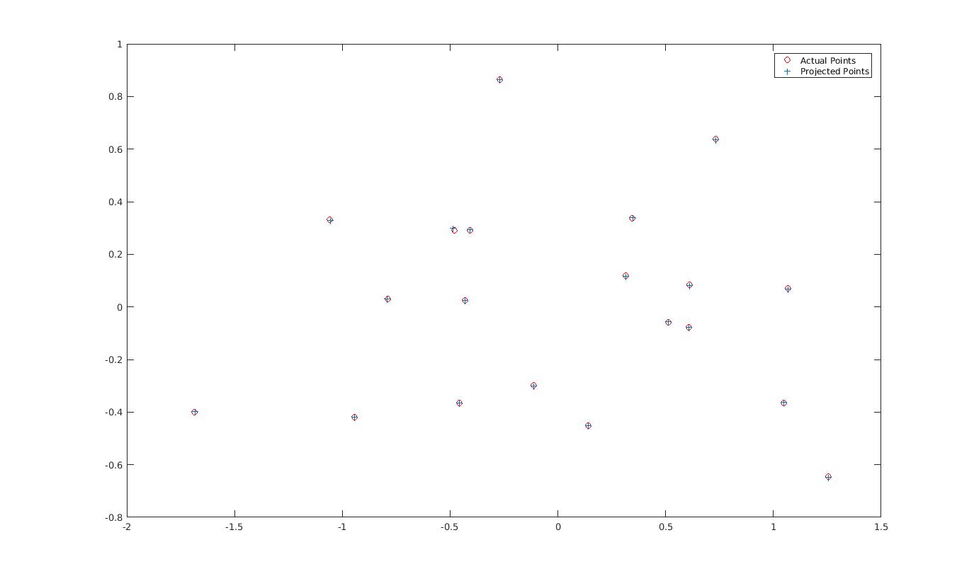
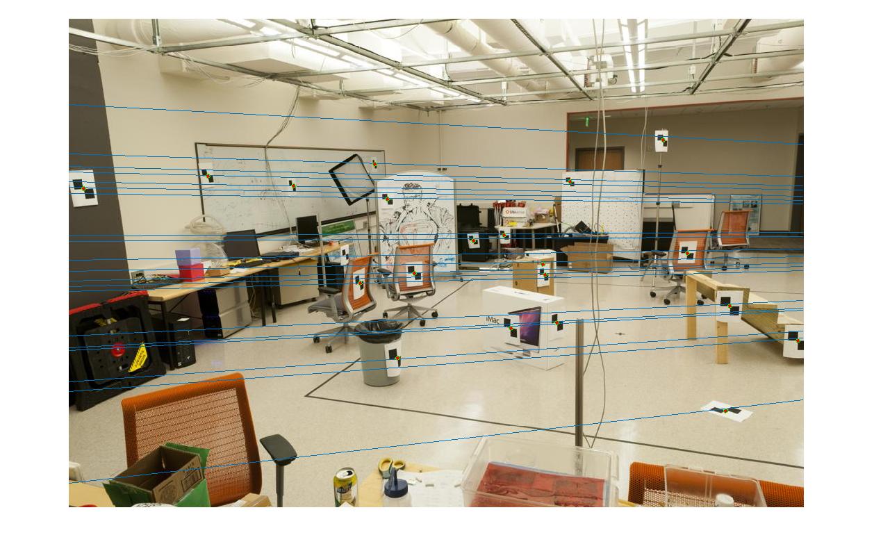
which normalizes the scale automatically. This approximate solution for F will be full rank, due to the problem formulation. Thus, we perform a second SVD and set the least singular value to 0, ensuring that F is rank two. This process ensures that the projected epipolar lines emanate from the same location. Fig. 2 shows epipolar lines produced via the approximated matrix F. In particular, the epipolar lines pass through the corresponding points, showing that the fundamental matrix has been correctly estimated.

Figure 2: Displys the estimated fundamental matrix F used to draw epipolar lines between two images of the same scene. The lines pass through the center of the related points, showing that F has been closely approximated.

The estimated matrix F is given by

⌊ ⌋ 0 0 − 0.0004 F = ⌈0 0 0.0034⌉ . 0 − 0.0046 0.1082

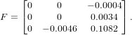(9)

Note that the graduate credit coordinate normalization has been applied before calculating this matrix.

3.2 Graduate Credit: Coordinate Normalization

To prevent numerical issues, one strategy is to perform a coordinate normalization between the two sets of points. We performed this utilization using the mean and standard deviation to estimate the scale of the image. These transformations for each set of points are given by

⌊ s 0 0⌋ ⌊1 0 − μx ⌋ T = ⌈ 0 s 0⌉ ⌈0 1 − μy⌉, 0 0 1 0 0 1

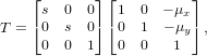(10)

where a separate T matrix is calculated for each set of points. Then, the normal fundamental matrix estimation is performed with this change of basis. After esimating F_norm, F is given by

T F = Tb FnormTa.

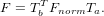(11)

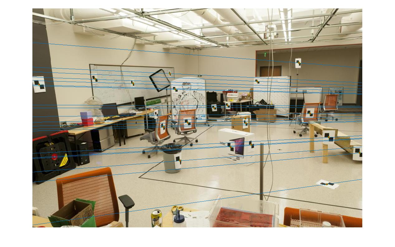
This normalization greatly improved the accuracy of the fundamental matrix approximation. Fig. 3 shows the operation of the fundamental matrix before the coordinate transformation. This process encounters numerical issues, causing the lines to pass by the corresponding points, decreasing the accuracy of the approximation. Fig. 2 displays the fundamental matrix calculated with the coordinate normalization.

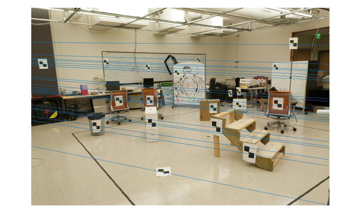
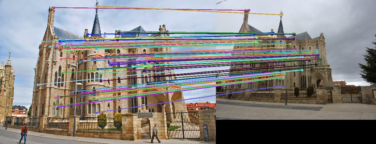
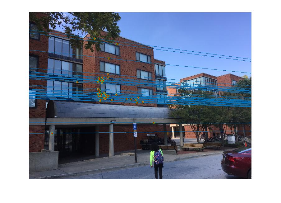
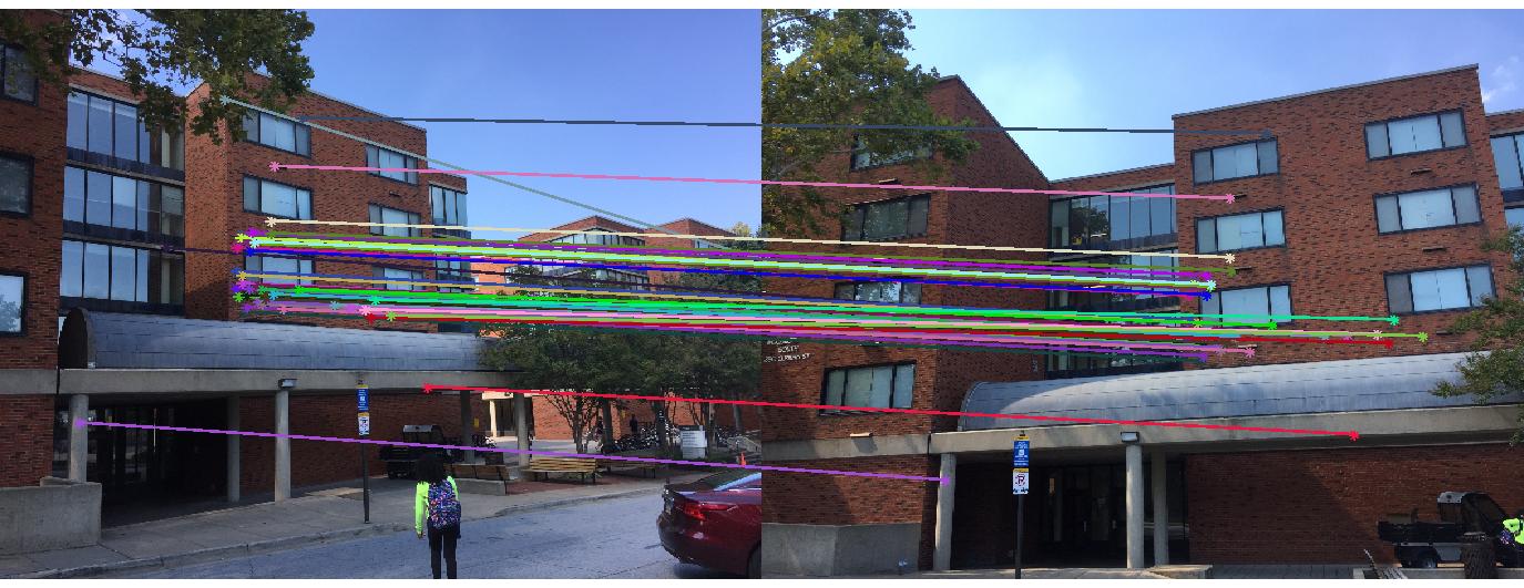
Figure 3: Displys the estimated fundamental matrix F used to draw epipolar lines between two images of the same scene. The lines do not pass through the center of the related points, showing that F is not well approximated without coordinate normalization.

4 Part Three

This portion of the assignment utilizes the RANSAC algorithm to perform feature matching between pairs of images. In particular, we discuss our RANSAC algorithm and present pairs of feature with points identified through inliers of the estimated fundamental matrix.

4.1 RANSAC

To perform our RANSAC algorithm, we select 8 points at random from the pairs and count the number of ”inliers” that agree with this particular matrix. To determine the inliers, we utilize the ”distance” metric

d(x′,x) = ∘ |x′F-x|

(12)

and take all inliers such that

d(x′,x) ≤ c,

(13)

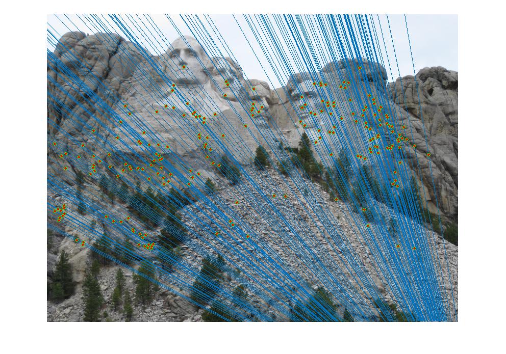
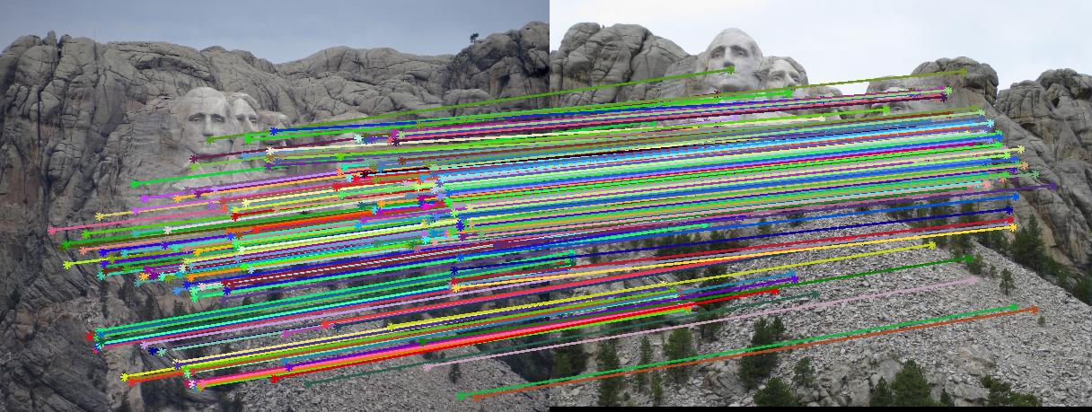
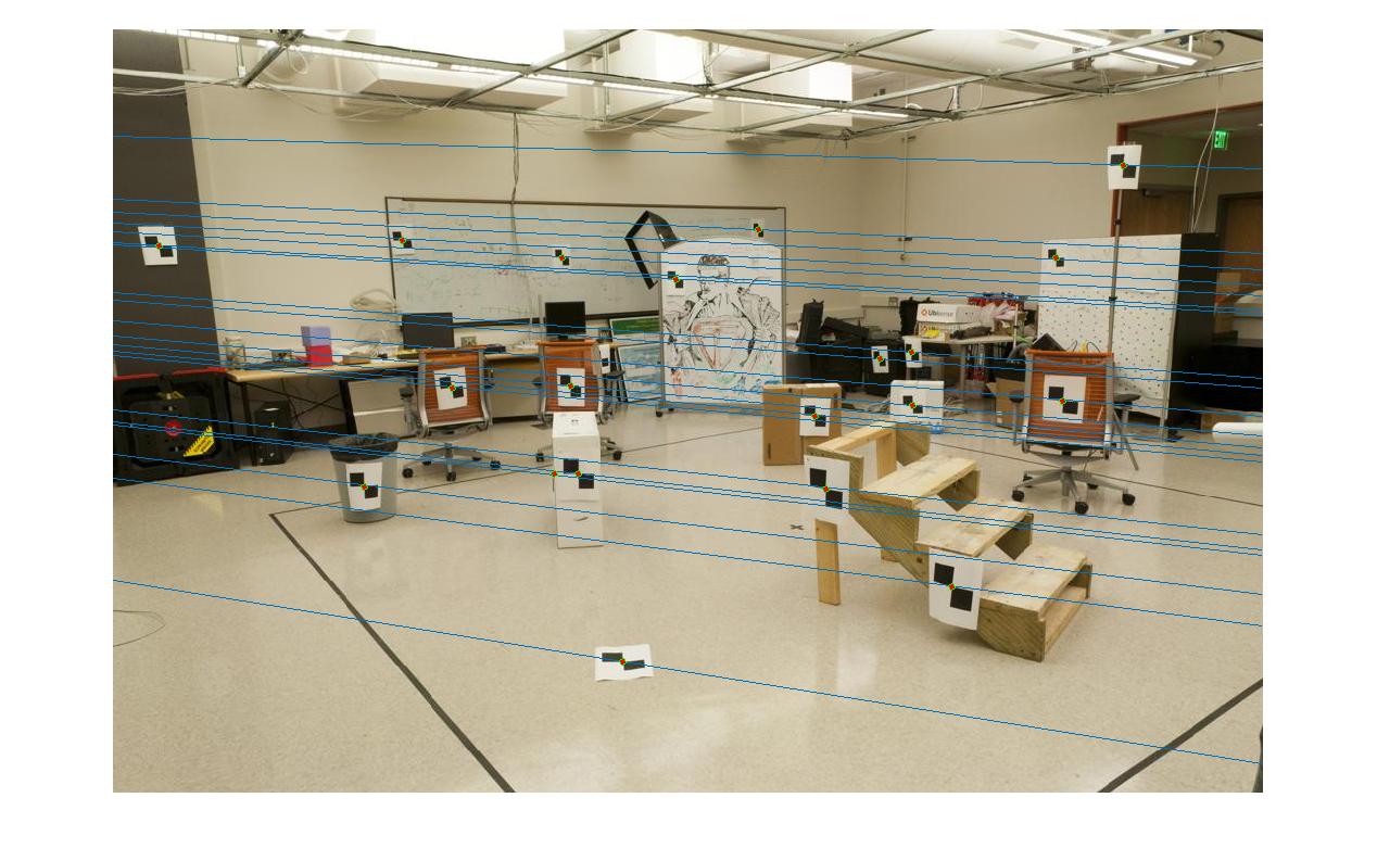
where c ∈ R⁺ is some constant. After several thousand iterations, we return the fundamental matrix with the most inliers and the inliers. Figs. 4,5 display the results of the RANSAC algorithm on the Notre Dame image pair. Even with these planar images, the RANSAC-estimated fundamental matrix allowed the algorithm to achieve 99% accuracy.

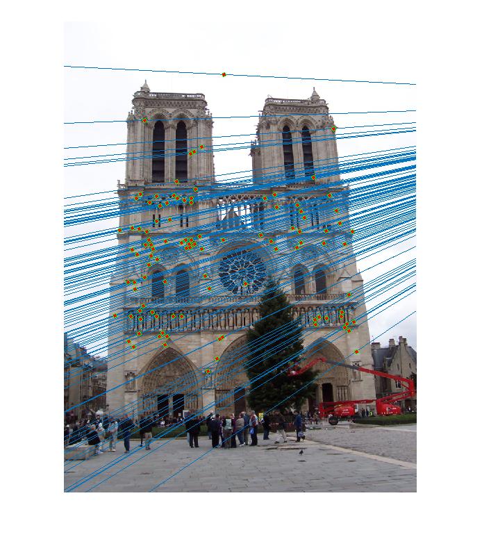
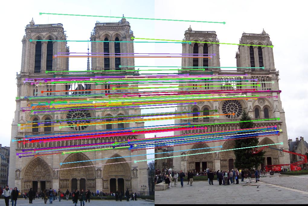
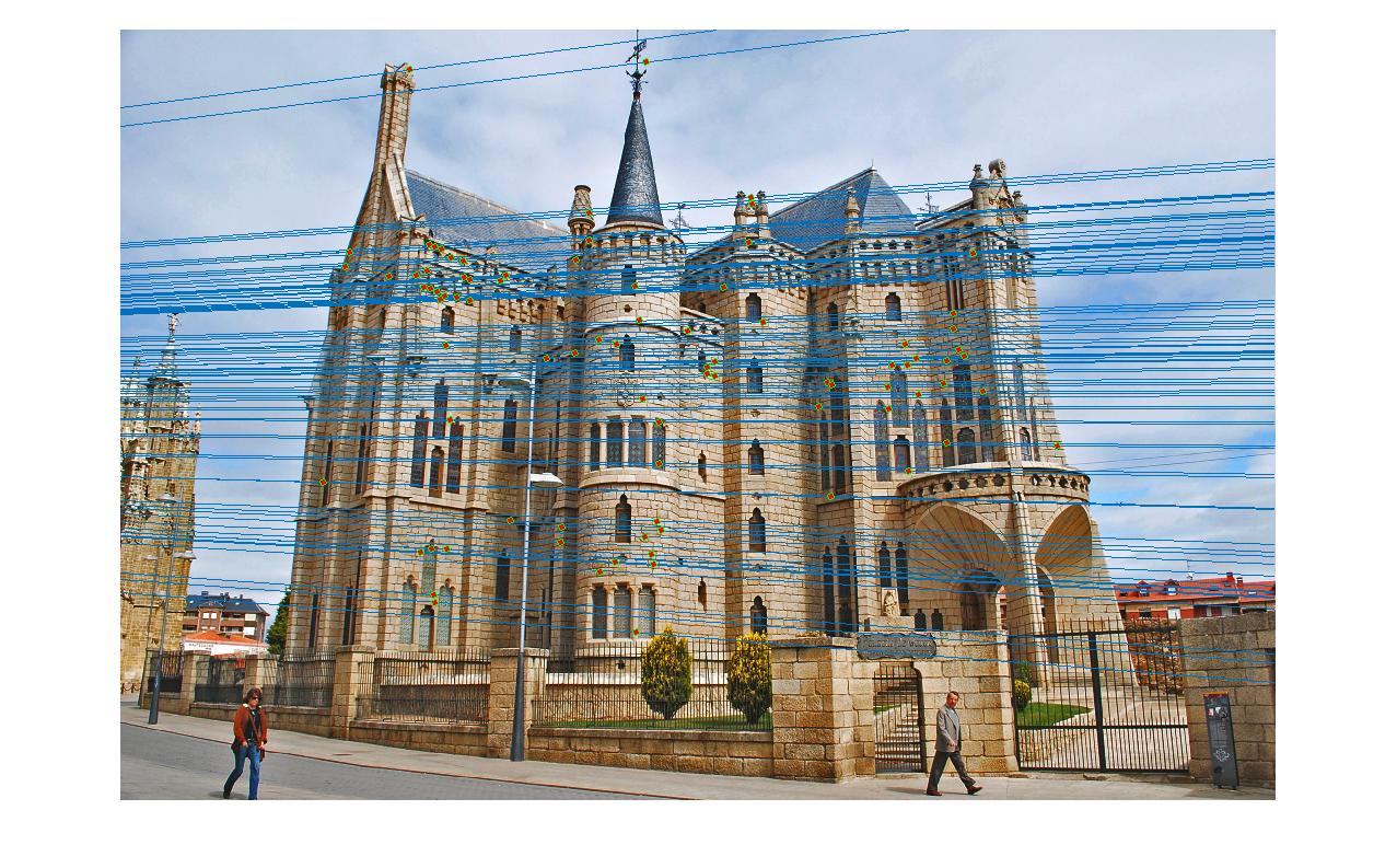
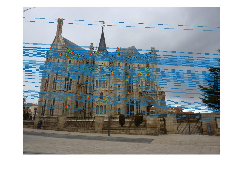
Figure 4: Displays the epipolar lines and inliers for an estimated fundamental matrix F on the Notre Dame image pair. The inliers for the estimated matrix were matched to the corresponding image with 99% accuracy.

Figure 5: Displays the corresponding points (i.e., inliers) for an estimated fundamental matrix F on the Notre Dame image pair. The inliers for the estimated matrix were matched to the corresponding image with 99% accuracy.

Figs. 7-11 display this matching on more of the supplied image pairs.

Figure 7: Displays the epipolar lines and corresponding inliers for the Mount Rushmore image pair.

Figure 9: Displays the epipolar lines and corresponding inliers for the Episcopal Gaudi image pair.

Figure 11: Displays the epipolar lines and corresponding inliers for the Woodruff dorms image pair.

5 Conclusion

This assignment proposed using linear least squares techniques to solve for the projection matrix and camera center between two known image pairs. Additionally, we estimated a fundamental matrix, which displays the epipolar geometry, between these pair of images. Utilizing coordinate normalization, we improved the results of this method. Finally, we utilized the RANSAC algorithm to approximate a fundamental matrix between an image pair amoung the presence of outliers. Using this method, 99% accuracy was achieved in finding corresponding image pairs.