Project 3: Camera Calibration and Fundamental Matrix Estimation with RANSAC
Contents
Example evaluation image
This project focused on camera calibration, the fundamental matrix, and ways in which we can extract information based on stereo correspondences between two images. It starts with a calculation of the project matrix between two images based on known points in space. Then, we derive the fundamental matrix for two images based on correspondences. Finally, we use this estimation to run the RANSAC method to find a best fundamental matrix for an image pair to better finding matches between the two images.
Algorithm Explanation
Each part of this project had it's own unique methods, although parts 1 and 2 were very similar in their form.
Calculating the Projection Matrix
The first part of this project focused on calculating the projection matrix between two images and then extracting the camera location. We do this by using a set of known correspondences between the two images, as well as their real 3D locations, in order to fit a model that represents our mapping between the world and camera coordinates. For this problem, there are two approaches to solving for the projection matrix. One is to use a linear regression with a fixed scale, and the other is to perform SVD on the matrix. Both algorithms are explained below.
The first part of the algorithm is almost identical for both linear regression and SVD. We first allocate some space for our A and b matrices, and then fill in our b matric with our 2D points. Next, we loop over the lists of points and extract their values into X, Y, Z, u, and v. We then progress by setting up our A matrix for each pair or correspondences following the given formula. For regression, each row is 11 elements, while for SVD, we would actually want to have each row be 12 elements. In the case of SVD, we would append a -u at the end the first row and -v at the end of the second for each loop iteration, making sure the allocated size of A was Nx12 instead of Nx11.
A = zeros(size(Points_2D,1)*2, 11);
B = zeros(size(Points_2D,1)*2, 1);
B(1:2:end,:) = Points_2D(:,1);
B(2:2:end,:) = Points_2D(:,2);

for i=1:1:size(Points_2D, 1)
   X = Points_3D(i,1);
   Y = Points_3D(i,2);
   Z = Points_3D(i,3);
   u = Points_2D(i,1);
   v = Points_2D(i,2);

   A(i*2-1,:) = [X,Y,Z,1,0,0,0,0,-u*X,-u*Y,-u*Z];
   A(i*2,:) = [0,0,0,0,X,Y,Z,1,-v*X,-v*Y,-v*Z];
end
To solve for the matrix, we have the first option of doing a linear regression. The code for this is below. We simply use Matlab's built in solver with the '/' operator to solve for 'M', where M is our projection matrix. We then have to set the last element in the matrix to 1.0 since we had to fix the scale.
XM = A\B;
M = vec2mat(XM,4);
M(3,4) = 1.0;
The calculated projection matrix for this method had a residual of .0445:
% Projection matrix for linear regression
 0.7679   -0.4938   -0.0234    0.0067
-0.0852   -0.0915   -0.9065   -0.0878
 0.1827    0.2988   -0.0742    1.0000
The other option is the SVD method. For this, we simply calculate [U,S,V] by doing the SVD of A, and then extract our matrix 'M' from the last column of V. We then resize this vector into a matrix to get our final matrix
[U,S,V] = svd(A,0);
M = vec2mat(V(:,end),4);
The calculated projection matrix for this method had a residual of .0445:
% Projection matrix for SVD
 0.4583   -0.2947   -0.0140    0.0040
-0.0509   -0.0546   -0.5411   -0.0524
 0.1090    0.1783   -0.0443    0.5968
After extracting the projection matrix, we are able to calculate the camera center. The code for this is quite simple:
Q = M(:,1:3);
m_4 = M(:,4);

Center = (-inv(Q))*m_4;
The final produced camera center for both regression and SVD are shown below:
% Linear regression camera center
<-1.5126, -2.3517, 0.2827>

% SVD camera center
<-1.5127, -2.3517, 0.2826>
Fundamental Matrix Estimation
The second part of the project was to estimate the fundamental matrix for a set of correspondences. This was based on the 8-point alogrithm detailed in class. We want to take our two sets of points and build a system of equations in order to solve for our fundamental matrix.
First, we need to set up our system of equations. In this case u_ and v_ correspond to the u' and v' needed, however using " ' " on a vector or matrix is the transpose in Matlab. For each set of points, we want to add a row to our A matrix. Once this is complete, we can run the SVD of A.
A = zeros(size(Points_a,1),9);

for i=1:1:size(Points_a,1)
    u_ = Points_a(i,1);
    v_ = Points_a(i,2);
    u = Points_b(i,1);
    v = Points_b(i,2);

    A(i,:) = [u*u_, v*u_, u_, u*v_, v*v_, v_, u, v, 1];
end
Next, we have the two step process of calculating the SVD of A and then rank-reducing the final fundamental matrix. We first run SVD, where we only care about the V matrix. Like the projection, we just want to extract the last column of V and convert it to a 3x3 matrix. After this, we need to run SVD again, and then set S[3,3] to zero. Once we do this, we can remultiply to calculate the new F_matrix, which will have rank 2.
% Run SVD on A matrix and extract F_matrix
[~,~,V] = svd(A);
F_matrix = reshape(V(:,end), [3 3]);

% Rank-reduce the matrix and recalculate
[U,S,v] = svd(F_matrix);
S(3,3) = 0;
F_matrix = U*S*v';
The final fundamental matrix produced by this code without point normalization is as follows:
% Fundamental matrix estimation
-0.0000    0.0000   -0.0019
 0.0000    0.0000    0.0172
-0.0009   -0.0264    0.9995
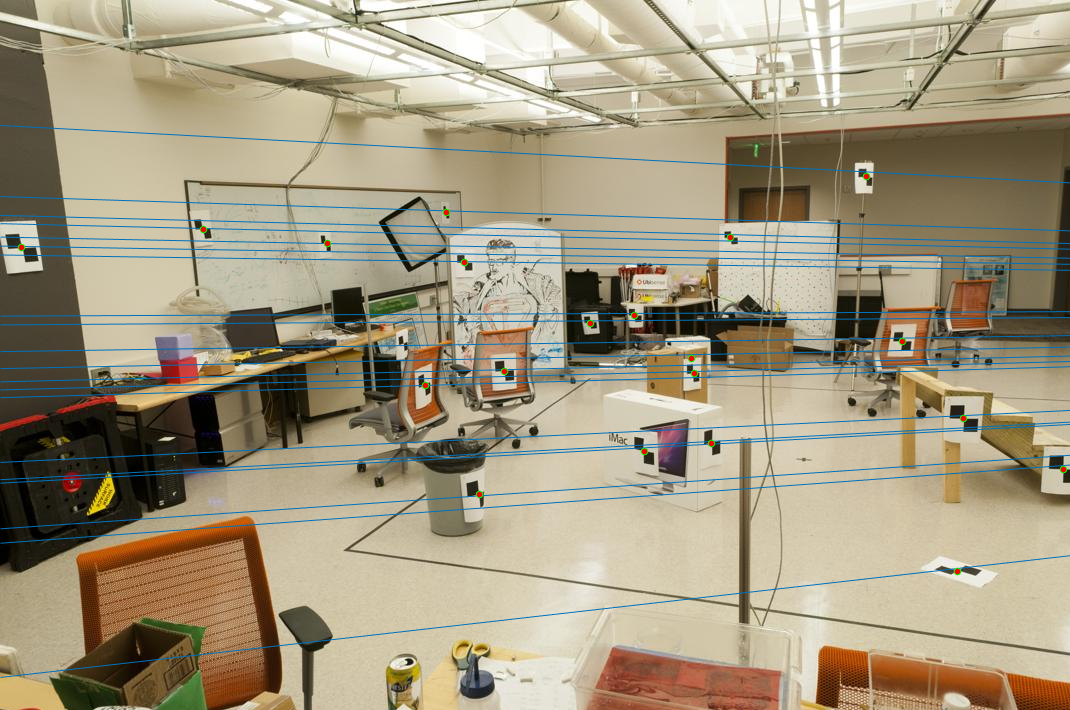
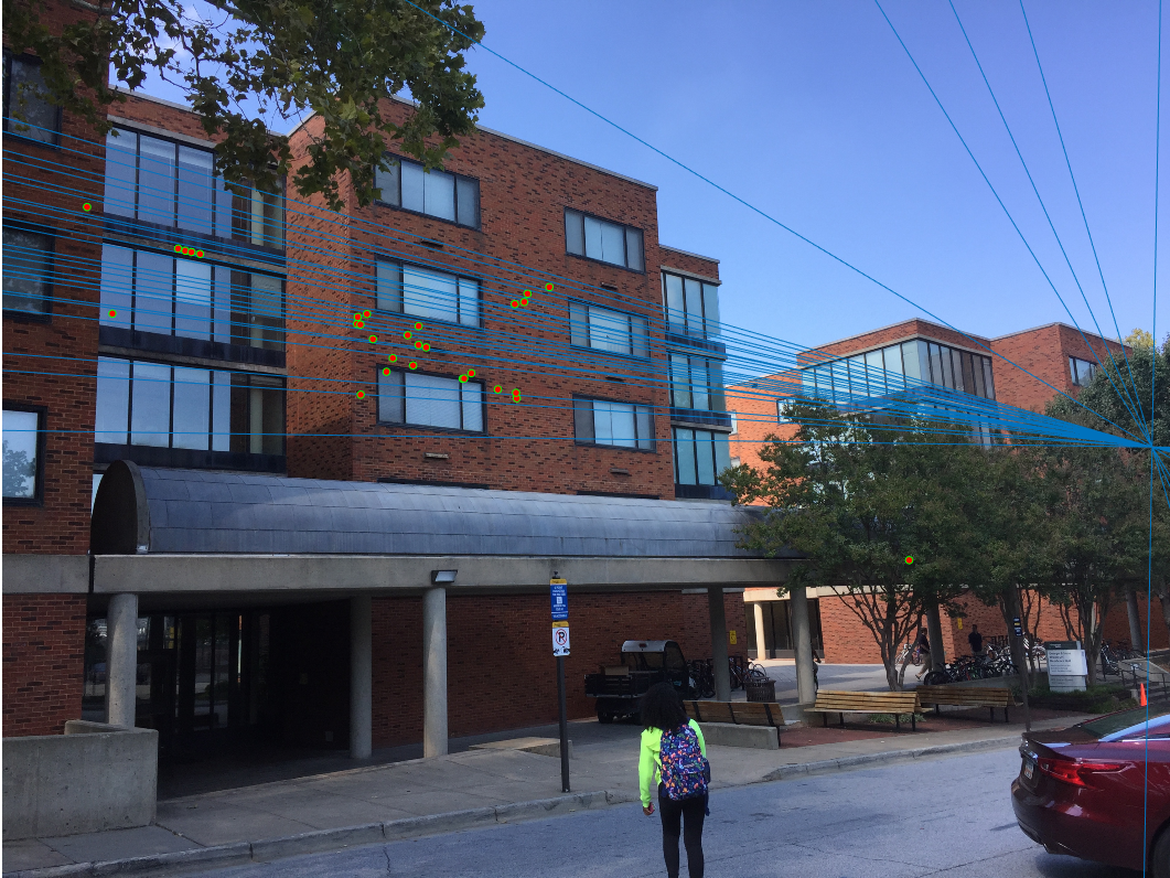
This produced the following epipolar lines:
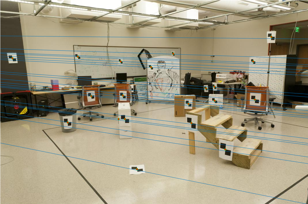
This was interesting, however, because the printed matrices before and after rank reduction were identical, but the blue epipolar lines perfectly passed through the centers of the points if no rank reduction occurred. After rank reduction, the lines were still good, but they were not perfectly through the center, even though the printed matrices were identical. This problem is later corrected by point normalization
RANSAC Fundamental Matrix Estimation
The final part of this project was to use the RANSAC algorithm in order to estimate a fundamental matrix for two images based on potentially corresponding matches between the two. From that point, we can find the set of inliers that best agree with each fundamental matrix to find the best matrix and also eliminate spurious matches from the list
To do that, we first set up some variables and matrices. The number of iterations can be calculated based on a specific formula, but for simplicity, I decided to hardcode the value 3000. Experimenting with different values for this showed that larger iterations generally performed better, but run time certainly increased. There are also some housekeeping variable to keep track of the inliers, as well as our threshold value. This value was very important when finding inliers. After some experimentation, I found that generally the range of [0.0045, 0.0075] worked quite well for most the of image pairs. This value can certainly be tuned greatly, and it's effects can be seen in the final results when checking for spurious points.
num_iterations = 3000;
point_indices = 1:size(matches_a,1);
threshold = .0075;
inliers_a = [];
inliers_b = [];
max_inliers = 0;
Best_Fmatrix = rand(3,3);
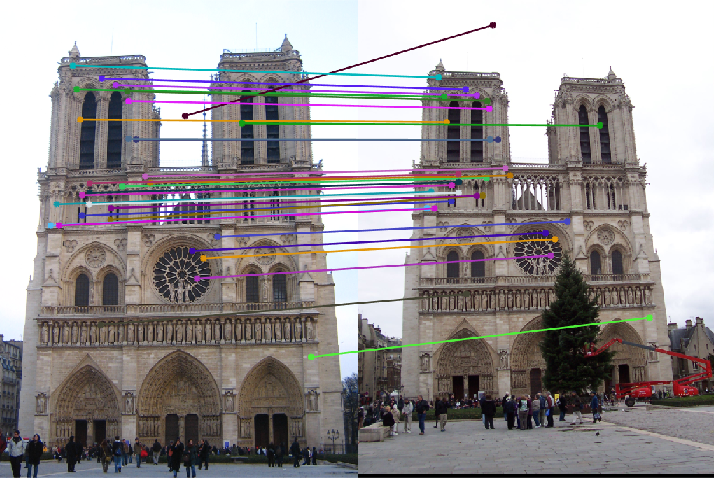
Next, we run our iterations of the RANSAC algorithm. First, we want to sample 8 random indices from the list of matches. We can then calculate a fundamental matrix based on these points. Once we have our fundamental matrix, we have to find the inliers. I did this by using a simple distance metric. We know that x'*F_matrix*x = 0, so we want to judge our points based on how close to zero they are. We calculate this value for each match from the entire set, and only save it in the inliers if it's absolute value is below our threshold. We can then check if we have a new best matrix, in which case we want to update our best model. Finally, rather than just take the first 30 points, I decided to randomly sample 30 points from our inliers as the matches to display.
for i=1:1:num_iterations

    indices = randsample(point_indices, 8);

    % Calculate our fundamental matrix for the 8 points
    F_mat = estimate_fundamental_matrix(matches_a(indices,:), matches_b(indices,:));
    num_inliers = 0;
    inliers = [];

    % Calculate the distance metric and save inliers
    for j=1:1:size(matches_a,1)
        xp = [matches_a(j,:), 1];
        x = [matches_b(j,:), 1];
        dist = abs(xp*F_mat*x');
        if dist < threshold
            num_inliers = num_inliers + 1;
            inliers = [inliers; dist, j];
        end
    end

    % Check if we have a new best F_matrix and set the values
    if num_inliers > max_inliers
        max_inliers = num_inliers;

        % Sort based on threshold
        % This is used to put the 'best' (closest to 0) matches in front
        inliers = sortrows(inliers);

        inliers_a = matches_a(inliers(:,2),:);
        inliers_b = matches_b(inliers(:,2),:);
        Best_Fmatrix = F_mat;
    end
end

s = randsample(1:max_inliers, 30);
inliers_a = inliers_a(s,:);
inliers_b = inliers_b(s,:);
RANSAC Results
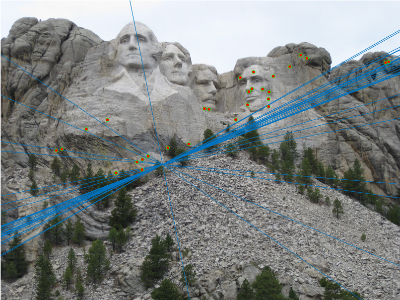
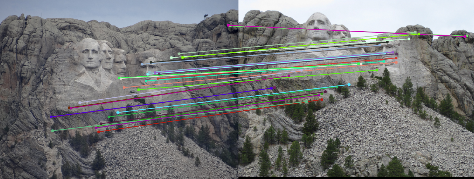
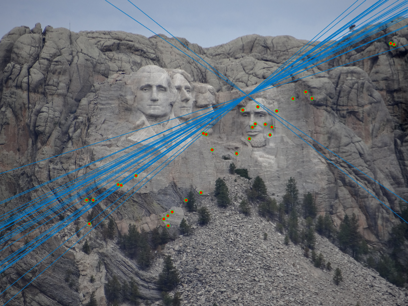
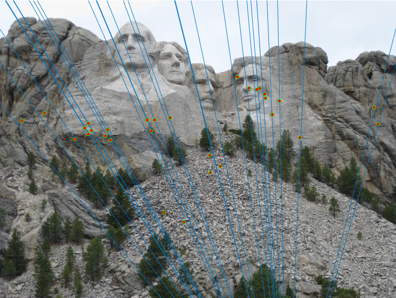
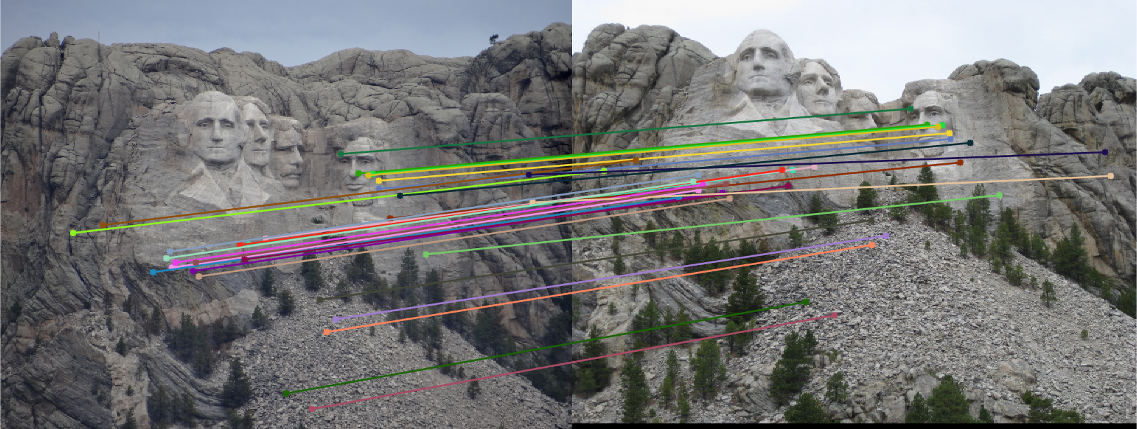
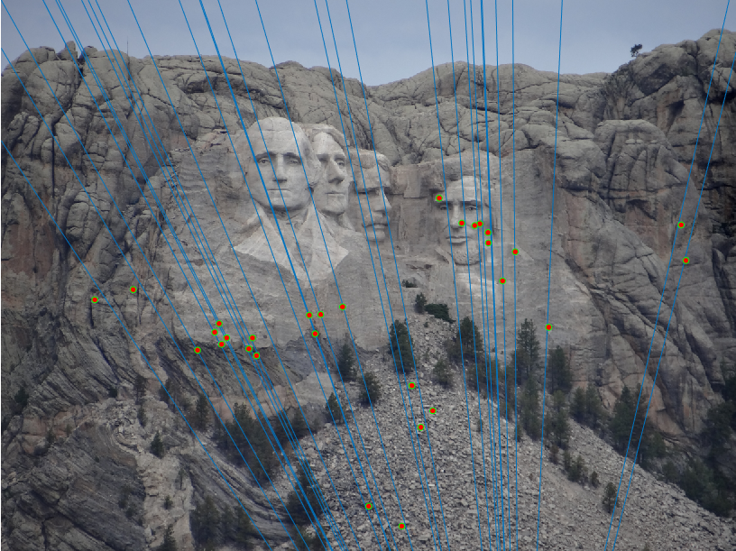
Without any point normalization, the results for the image pairs were overall 'okay'. The Mount Rushmore pair did quite well, resulting in the following epipolar lines and correspondence arrows. In this case, it seems that every inlier match found was correct, although the epipolar lines look quite incorrect.
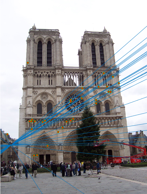
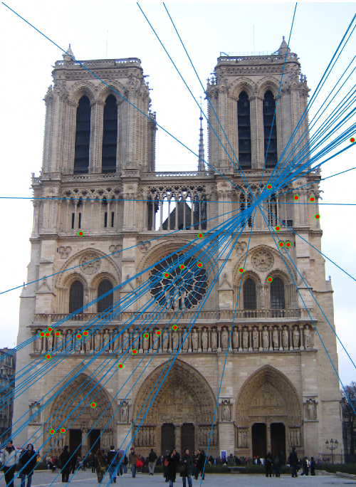
Other examples for the other image pairs can be seen below. The overall results were not quite bad as I expected. You can certainly tell that the fundamental matrix is not necessarily "correct", but it did function as a good estimation and decent way to remove our spurious matches
Point Normalization
As part of the extra credit for the 4476 section, I decided to implement a form of point normalization. The algorithm for this, as well as some comparisons for improvement can be seen below.
First, I decided to use the mean subtraction and standard deviation method to create the transformation matrices. To do this, I first took the mean of the list of points. This allows me to extract my c_u and c_v values. Next, I calculate a new list, p_a, that is simply the list of points with the corresponding mean subtracted. Once we have this new list, I calculate the standard deviation, and then take the reciprocal to get the scalar value we want for our transformation. The last step is to create our transformation matrix for this set of points. This is done by multiplying our 3x3 scalar matrix by our 3x3 matrix containing the c_u and c_v means. This is done for both Points_a and Points_b to get their translation matrices. We then simply apply the transformation matrix to each of the points in the corresponding lists. Finally, after calculating our fundamental matrix, we have to make sure to apply the transformation matrices to it as well.
norm_points = 1;
% Extra Credit to normalize all points for A and B
% Wrap in an if block so we can easily see difference when on and off
if norm_points

    % Calculate our transformation matrices by subtracting mean
    % then taking reciprocal of new standard deviation. We use these
    % values to build our final transformation matrix
    mean_a = mean(Points_a);
    cu_a = -mean_a(1);
    cv_a = -mean_a(2);
    p_a = [(Points_a(:,1)+cu_a), (Points_a(:,1)+cv_a)];
    std_a = 1./std(p_a);

    CA = diag([1 1 1]);
    CA(1,3) = cu_a;
    CA(2,3) = cv_a;
    Ta = diag([std_a(1) std_a(1) 1])*CA;

    mean_b = mean(Points_b);
    cu_b = -mean_b(1);
    cv_b = -mean_b(2);
    p_b = [(Points_b(:,1)+cu_b), (Points_b(:,1)+cv_b)];
    std_b = 1./std(p_b);

    CB = diag([1 1 1]);
    CB(1,3) = cu_b;
    CB(2,3) = cv_b;
    Tb = diag([std_b(1) std_b(1) 1])*CB;

    % Apply the transformation matrix to the points
    for i=1:1:size(Points_a,1)
       % This part looks a bit funky due to the double transpose
       a = (Ta*([Points_a(i,:) 1])')';
       b = (Tb*([Points_b(i,:) 1])')';
       Points_a(i,:) = a(1,1:2);
       Points_b(i,:) = b(1,1:2);
    end
end

% Fundamental matrix calculation from above goes here

% Apply transformation matrices
if norm_points
    F_matrix = Tb'*F_matrix*Ta;
end
This actually ended up fixing the issue with the epipolar lines in part 2 not passing perfectly through the center of the points. After adding this normalization method, a new fundamental matrix was produced, and the epipolar lines passed straight through the center of each point
% Fundmental matrix with Normalized Points
-0.0000    0.0000   -0.0003
 0.0000   -0.0000    0.0024
-0.0000   -0.0033    0.0779

Results
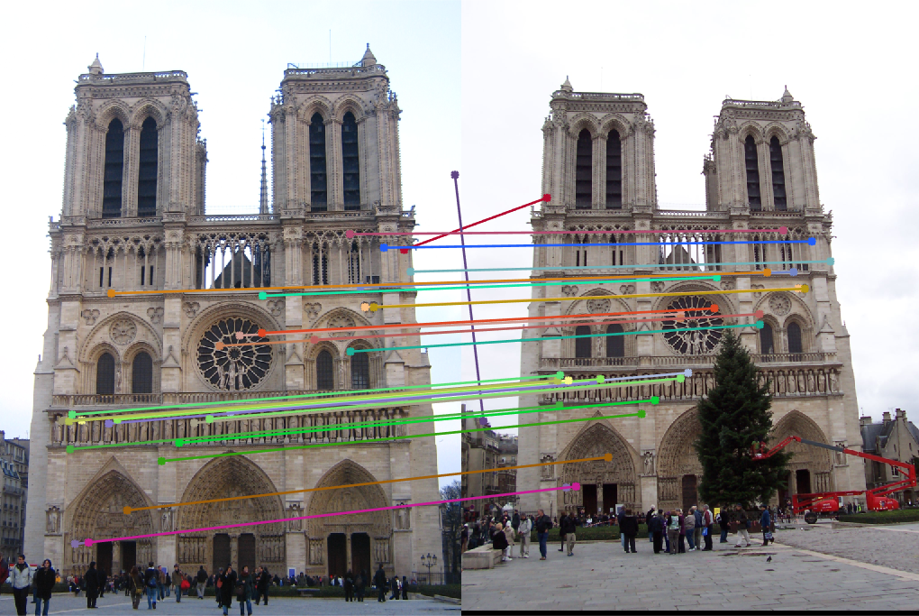
Direct comparison of epipolar lines before and after normalization can be seen following these sets
In the case of Rushmore, we can immediately see that the epipolar lines seem to make a bit more sense based on the movement of the camera. Also, 100% of the matches displayed here seem to be correct
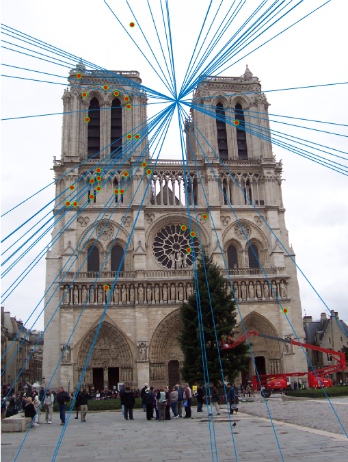
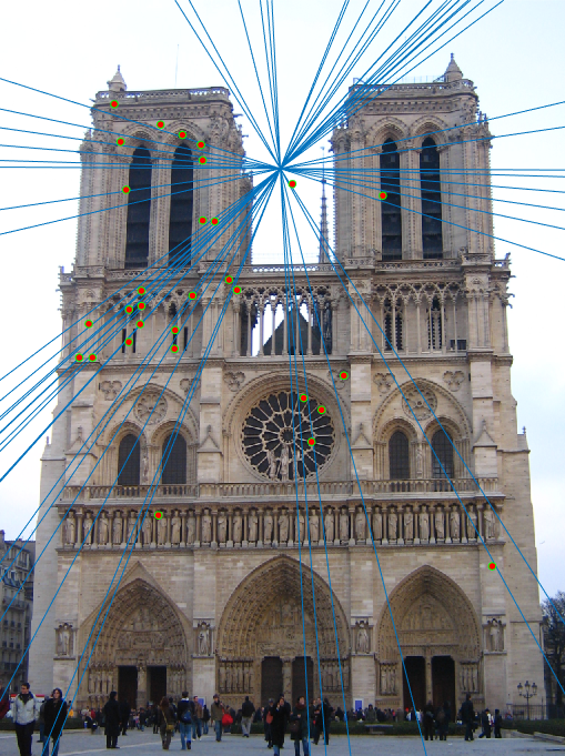
For the Notre Dame pair, we still see some points may be a bit off, such as the sky match, but overall, the points are much more accurate, and the epipolar lines are more consistent with the translation of the camera in the two photos.
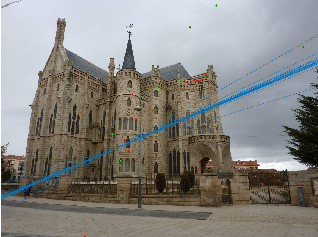
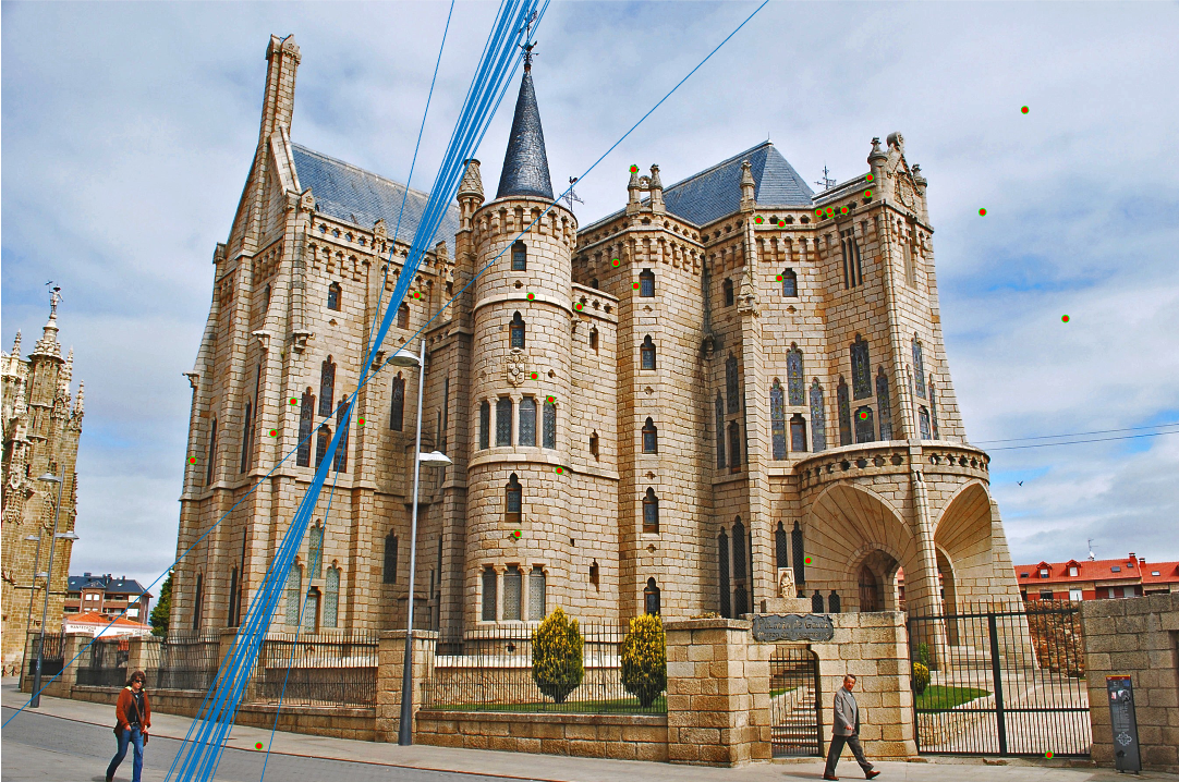
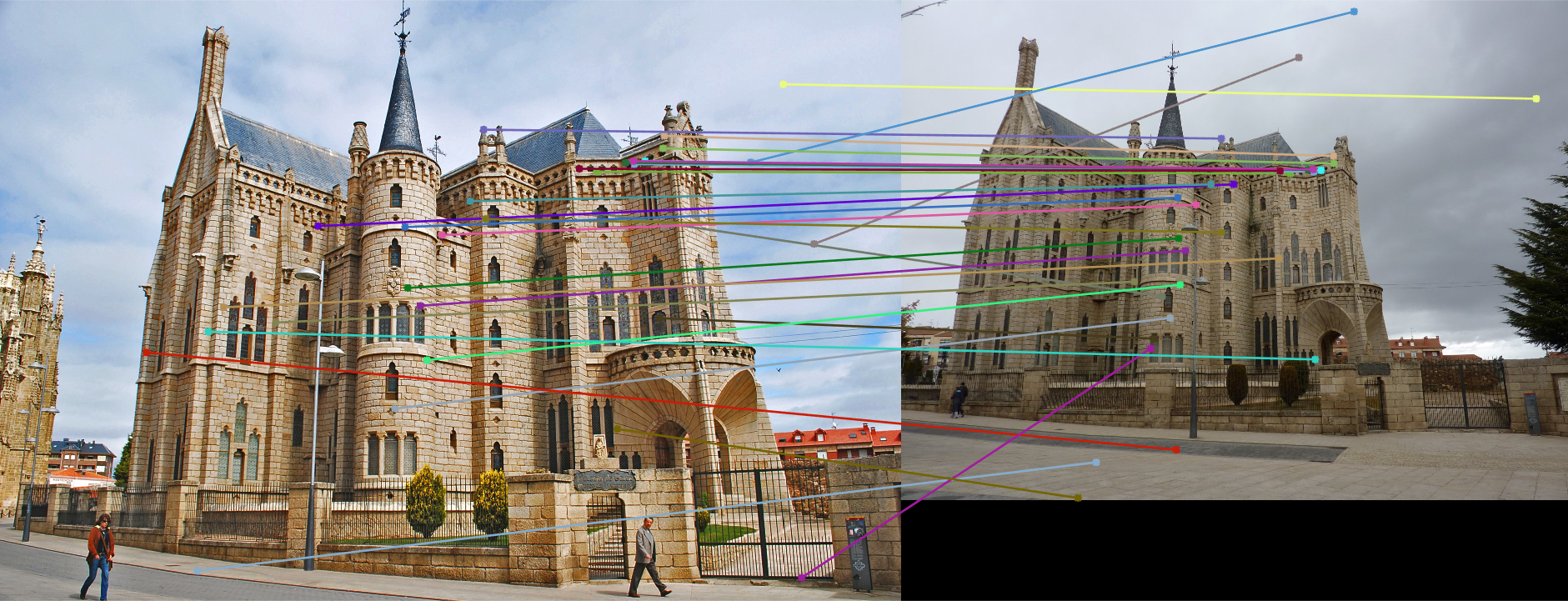
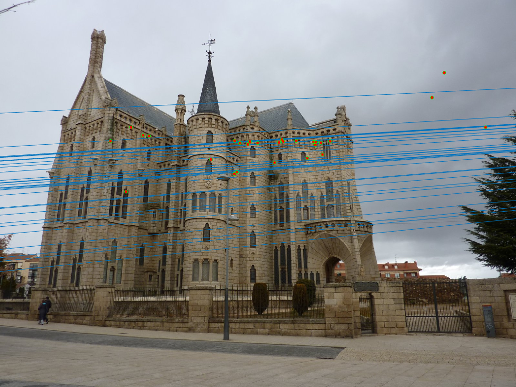
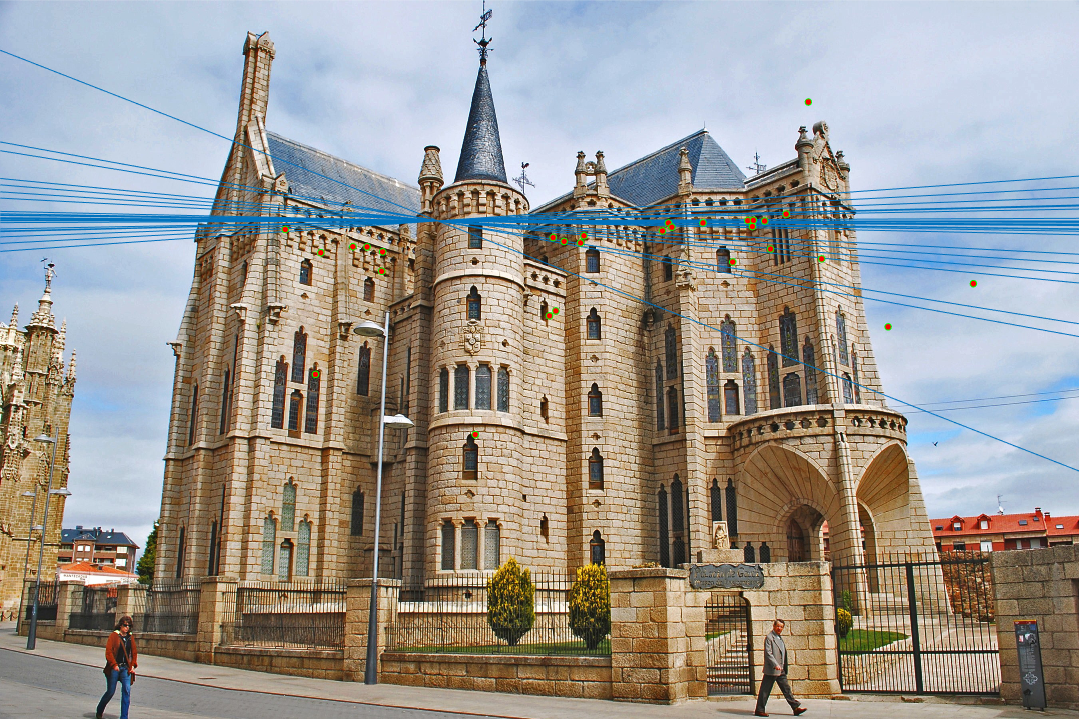
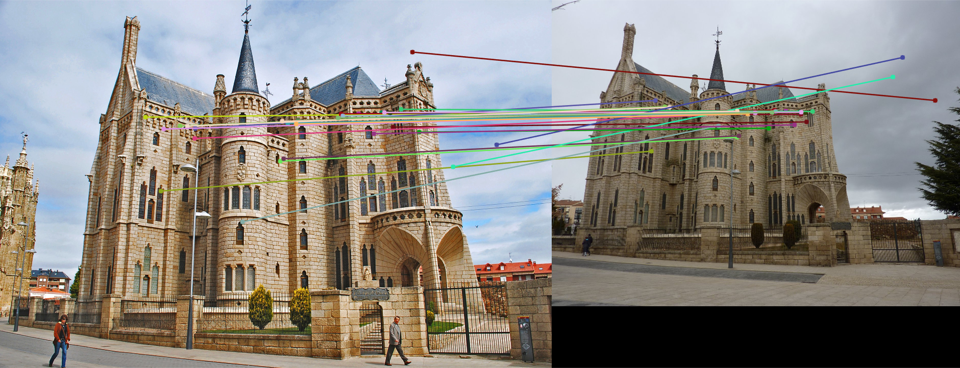
The method still struggled to find an amazing match for the Gaudi pair, however, it is still a significant improvement over the un-normalized points. We can see that with the normalized points, there are much fewer incorrect matches, and the epipolar lines seem more correct.
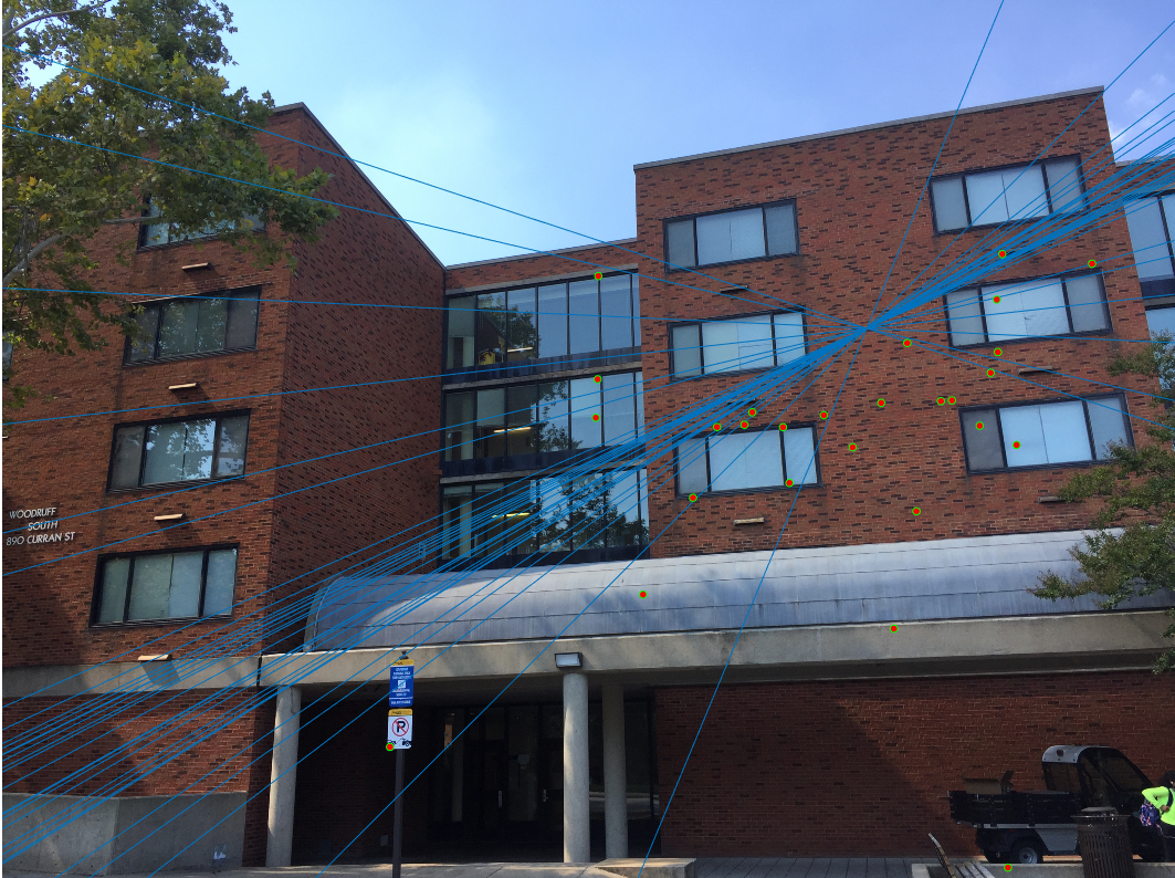
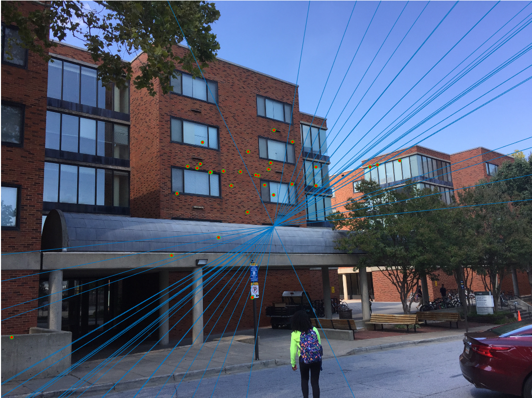
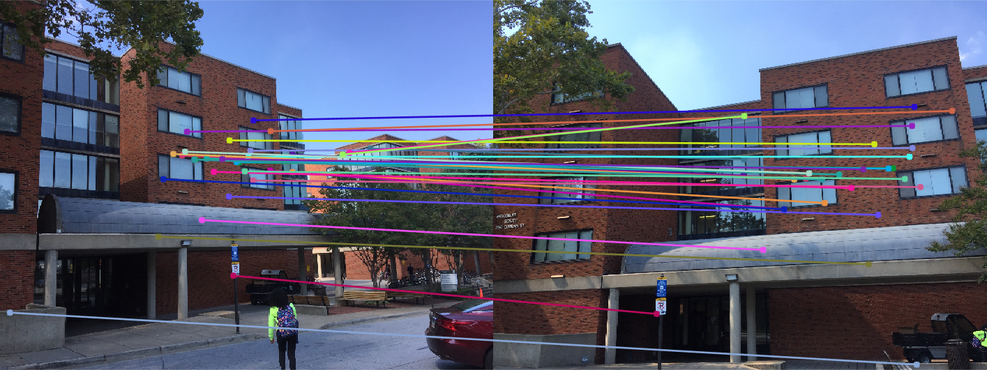
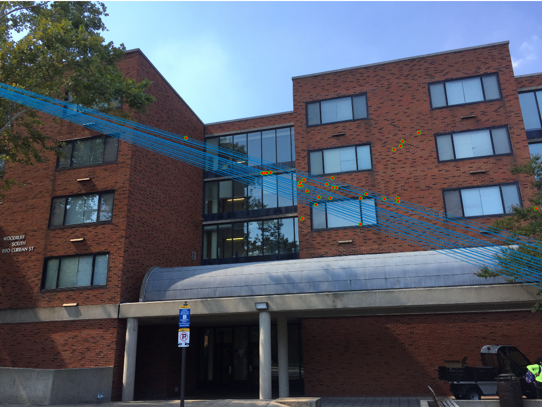
The Woodruff set also saw better results after normalization. There were much fewer incorrect matches, and the epipolar lines are more consistent
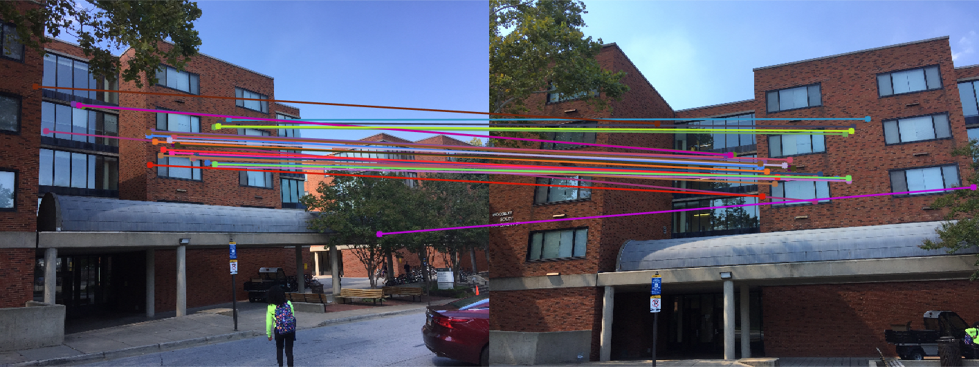
| Without Norm | With Norm |
|---|---|
|
|
|
|
|
|
|
|