Project 3: Camera Calibration and Fundamental Matrix Estimation with RANSAC
The goal of this assignment is to achieve the following 3 objectives
- Derive the components of the projection matrix that converts the world's 3D co-ordinates to 2D co-ordinates. This is evaluated to compute the residual between the projected location of each point in 2D from 3D and the actual location. Then, the camera center is computed.
- Estimate the mapping of points in one image to lines in another. This uses the fundamental matrix. The epipolar lines are then plotted to check the estimation.
- Estimate the fundamental matrix from data with noise using RANSAC along with the fundamental matrix estimation from part 2.
Part 1
This is how I derived the camera center. These are the following steps
I built an approximation matrix by utilising the equations below. This equation better illustrates the steps above.
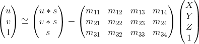
Since the final column of the matrix contains the world center after rotation as well as the application of the camera parameters as captured in the intrinsic matrix, I used this to derive the camera's center. The following equation depicts it clearly.
The projection matrix is:
0.7679 -0.4938 -0.0234 0.0067
-0.0852 -0.0915 -0.9065 -0.0878
0.1827 0.2988 -0.0742 1.0000
The total residual is: <0.0445>, which is pretty low.
The estimated location of camera is: <-1.5126, -2.3517, 0.2827>
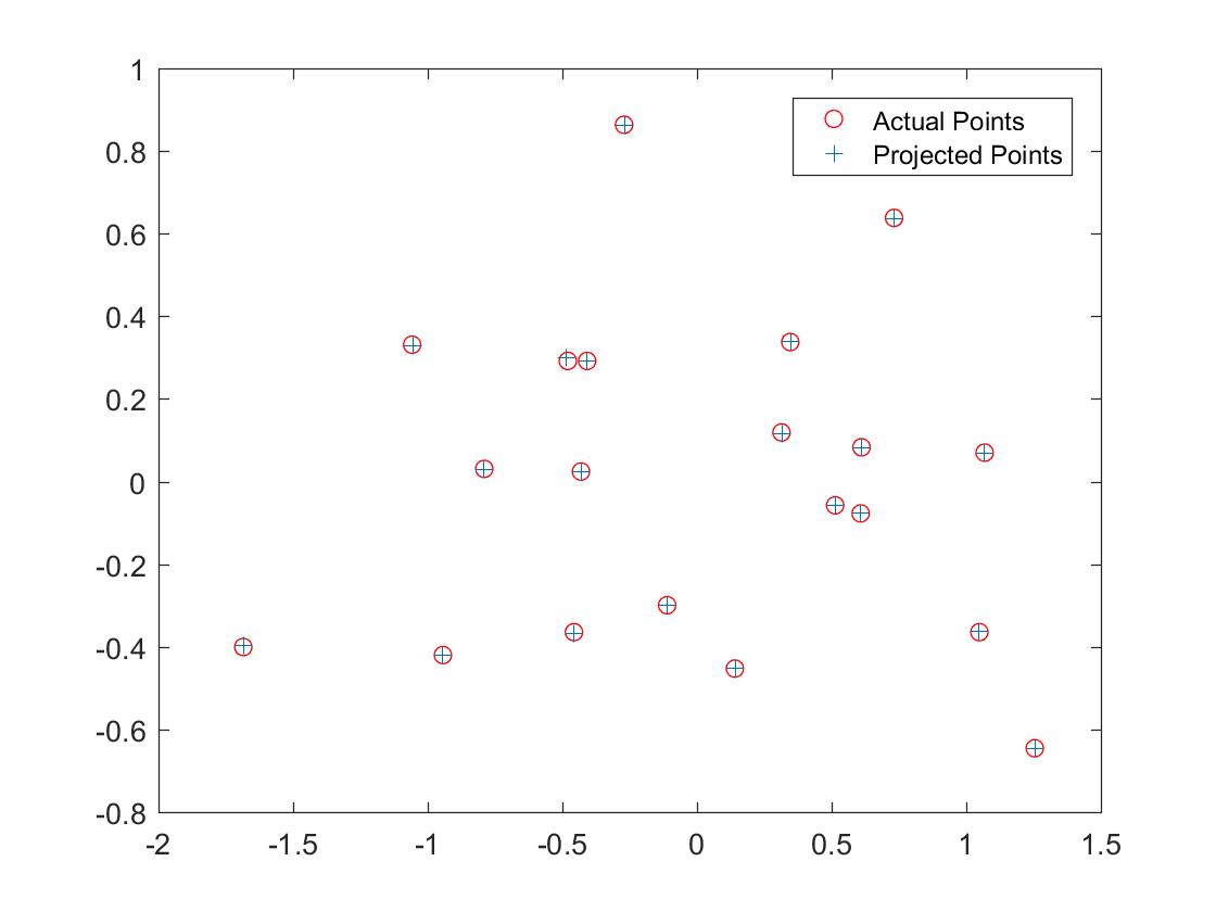
Projected and actual locations of points 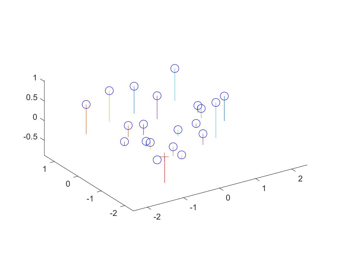
Point locations in the world and camera locations (cross) |
Part 2
This part was on deriving the fundamental matrix
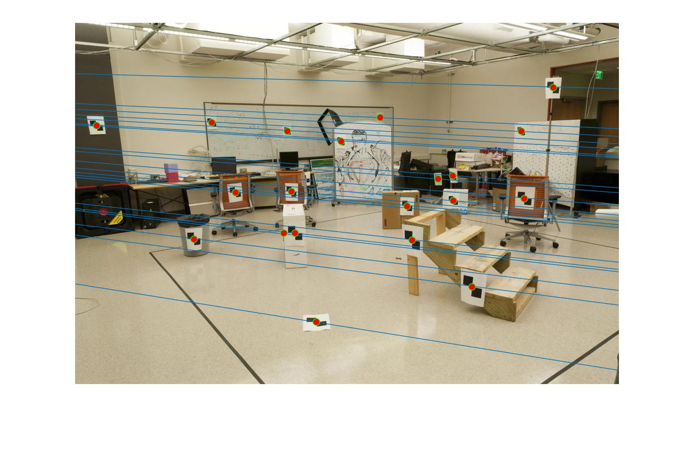
Epipolar lines on the first image 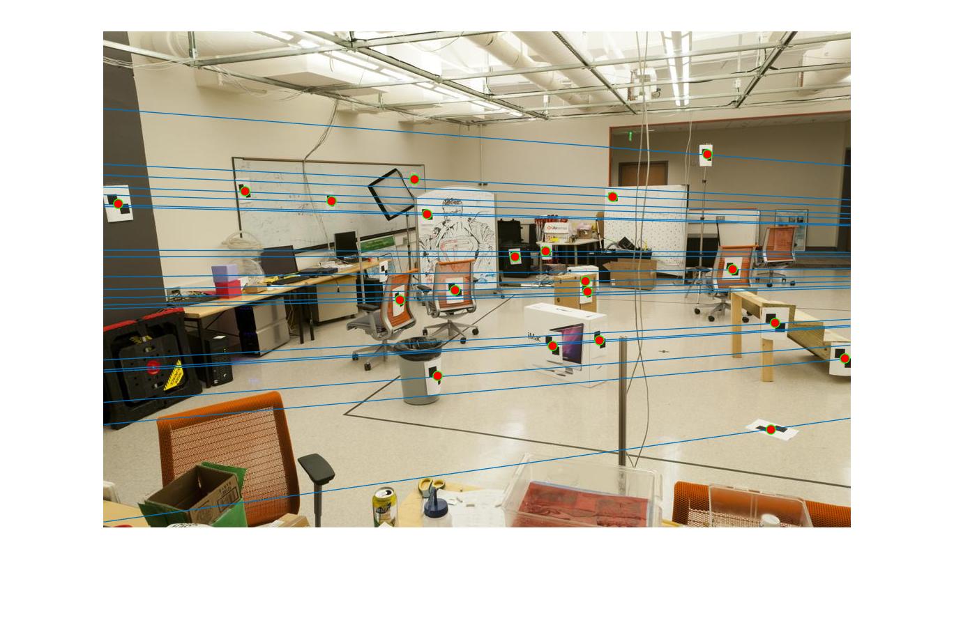
Epipolar lines on the second image |
The fundamental matrix is as seen below:
7.32379750235769e-06 -9.65627056161648e-05 0.0243514316332319
-6.06106618327418e-05 1.84673478184292e-05 -0.191366205380325
-0.000592583773105209 0.259444799071952 -5.24601919532604
Part 3
This part was on using RANSAC to estimate the fundamental matrix.
The results are as seen below
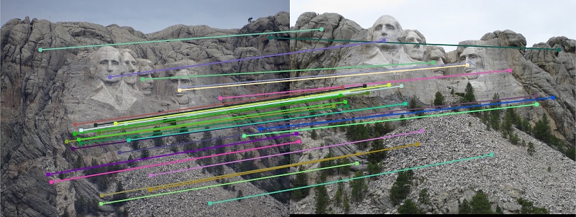
Epipolar lines with accuracy of 82%
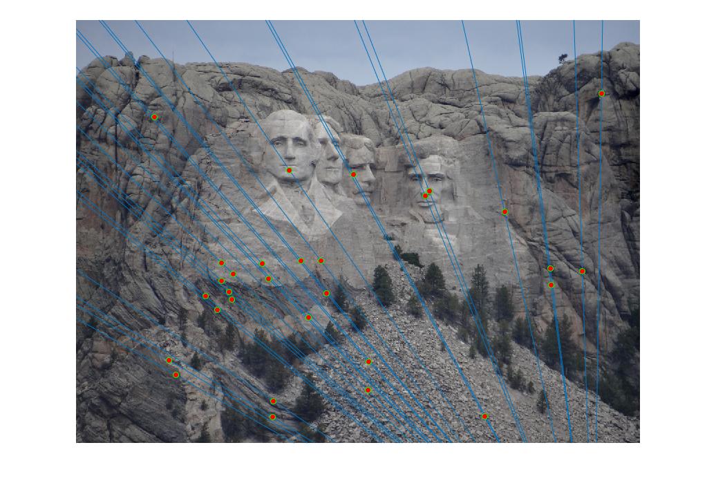
Results for mount rushmore with most confident fundamental matrix
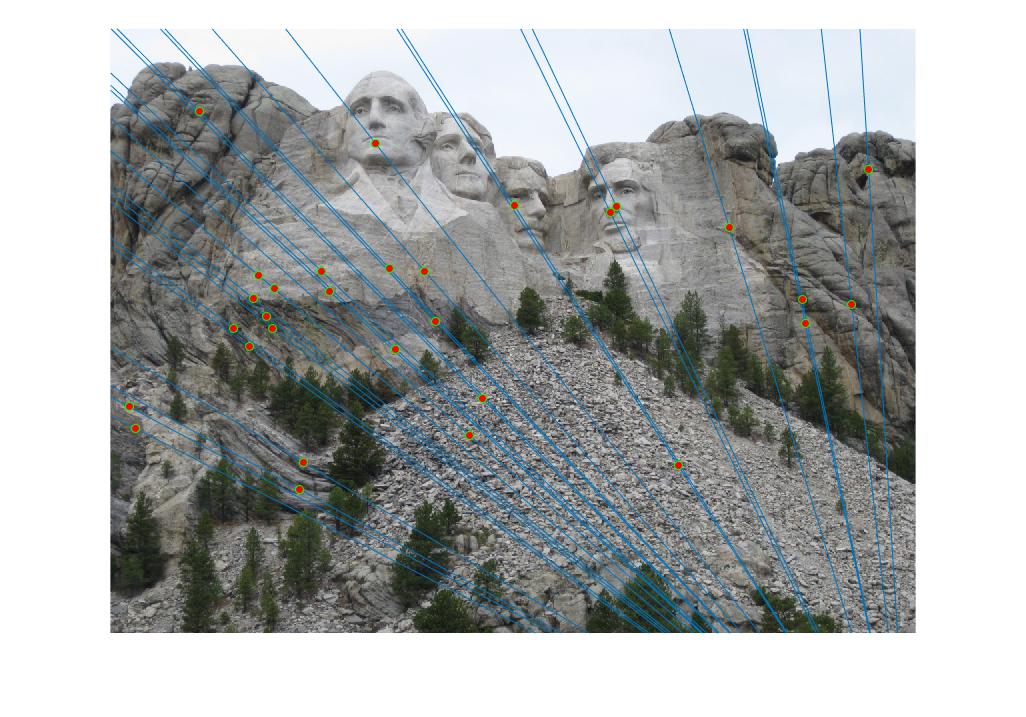
Results for mount rushmore with most confident fundamental matrix
Other images
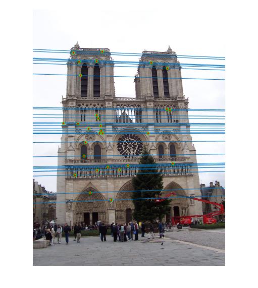
Results for notre dame with most confident fundamental matrix
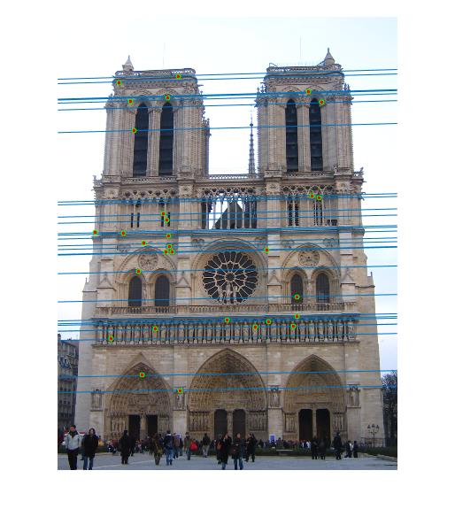
Results for notre dame with most confident fundamental matrix
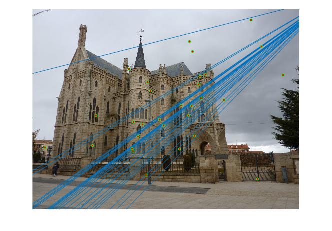
Results for episcopal gaudi with most confident fundamental matrix
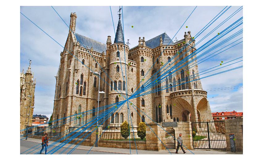
Results for episcopal gaudi with most confident fundamental matrix
Extra credit
For extra credit, I normalized the points in the image co-ordinates. Since the equation modelled by the matrix that produces the fundamental matrix relies on the multiplication of the point co-ordinates, the produced values differ greatly and the matrix of point correspondences is sensitive to error. When normalized, they are less likely to vary strongly.
As far as implementation goes, I estimated the standard deviation of the points as the square root of 2. I then adjusted them based on the center and the standard deviation ratio. This is a code snippet to illustrate a general skeleton of how I performed my normalization. The rest of the implementation is in estimate_fundamental_matrix
        standardize_a = std(Points_a(:,1) - col_mean_a(1)) + std(Points_a(:,2) - col_mean_a(2));
        singular_a = diag([1, 1, 1]);
        singular_a(1) = coefficent / standardize_a;
        translation_a = singular_a * col_mean_prime_a;
        normalized_points_a = (translation_a * Points_a')';
The results are illustrated with episcopal gaudi as seen below in a before and after picture.
|
Scene a without normalization |
Scene b without normalization |
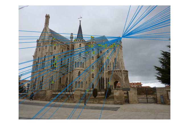
Scene a with normalization |
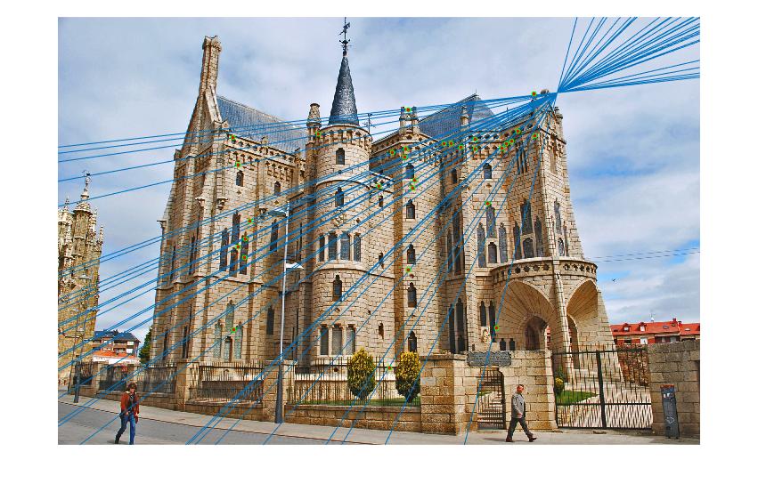
Scene b with normalization |
As can be clearly seen, episcopal gaudi had performance that was not as good as the other images before and after both, but after normalization, the performance increased and my extra credit normalization section worked!