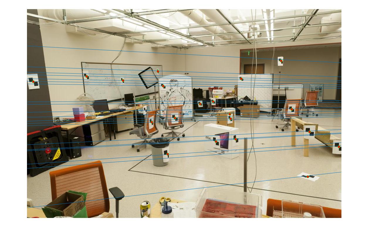
Project 3 / Camera Calibration and Fundamental Matrix Estimation with RANSAC
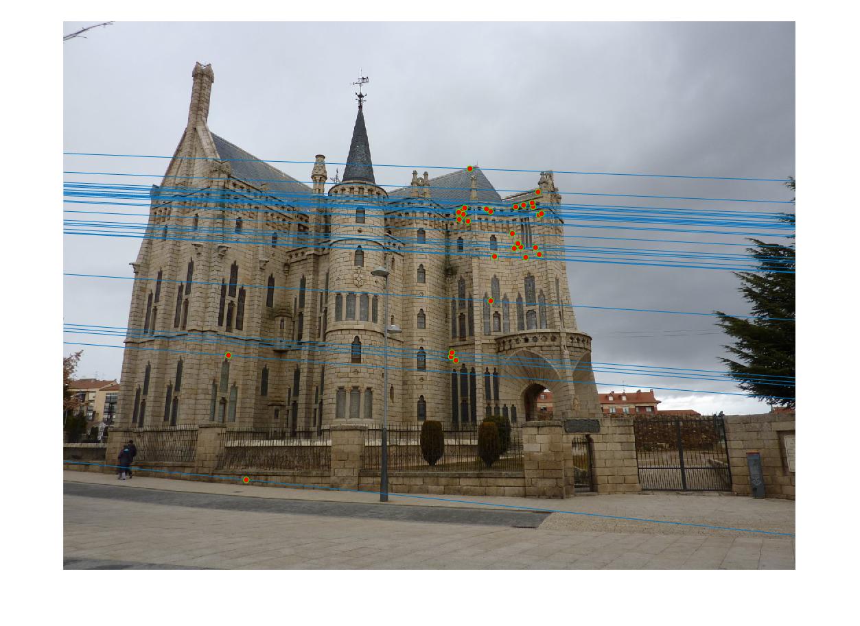
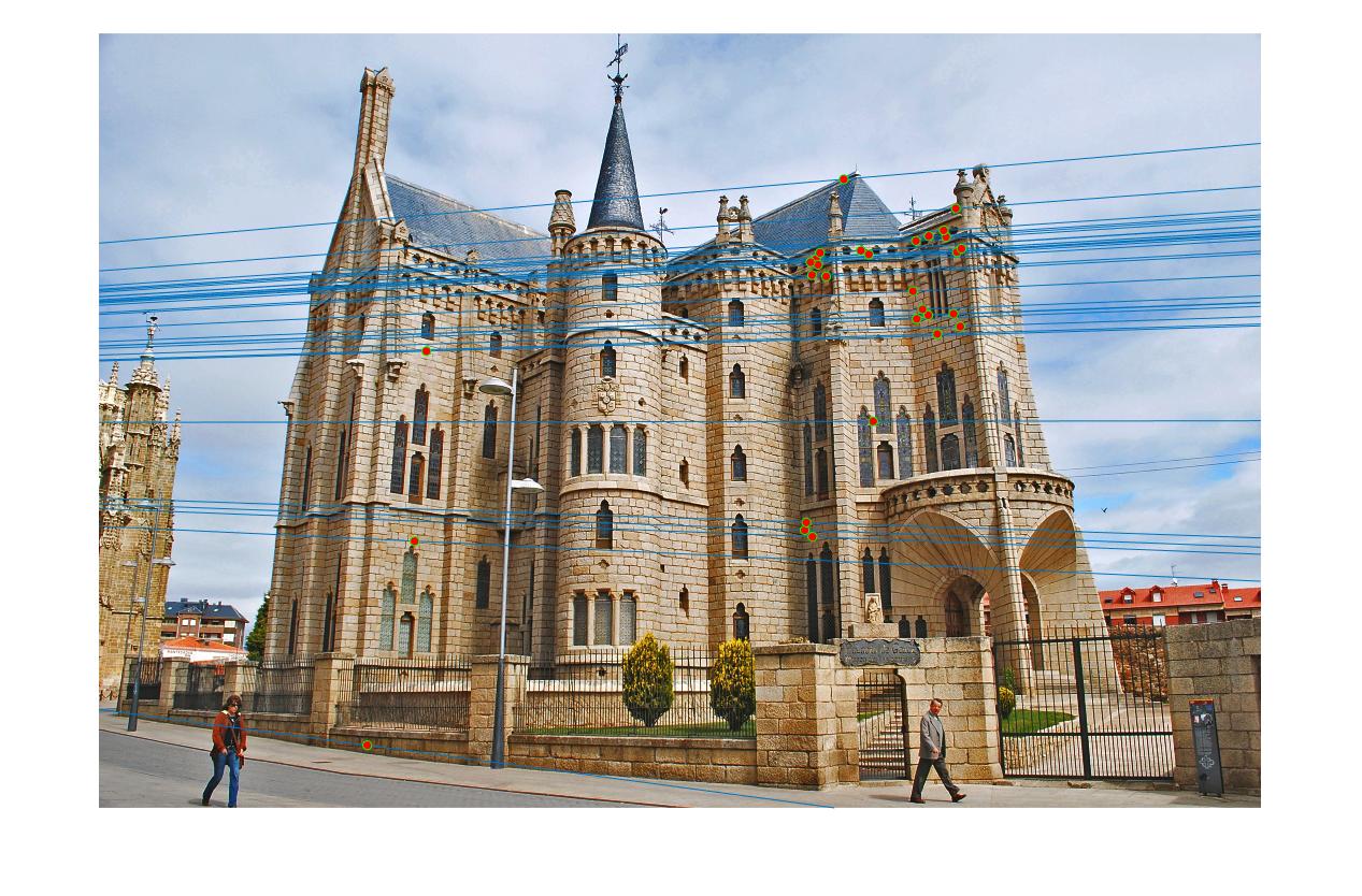
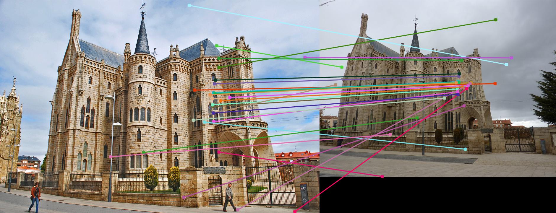
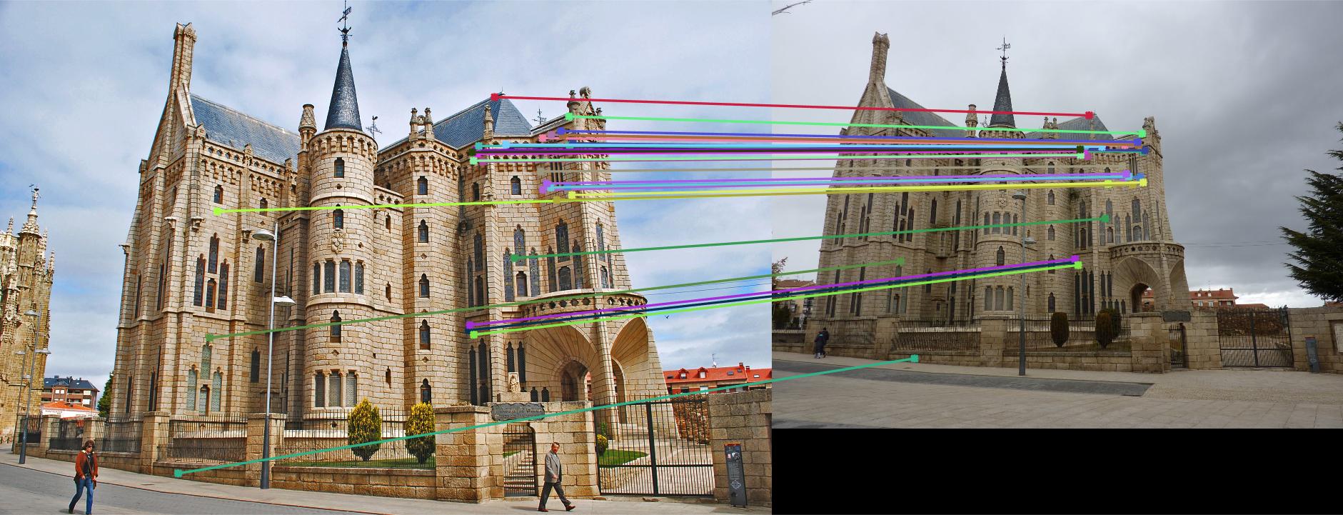
The epipolar lines for 30 inliers after normalization on Episcopal Gaudi
The implementation contains 3 important steps:
- Camera Projection Matrix
- Fundamental Matrix Estimation including normalization
- Fundamental Matrix with RANSAC
The follwing description includes the implementation and the results of algorithm I have used for all the parts.
Camera Projection Matrix
In compute_projection_matrix() I intially create an array given the 2D and 3D datapoints to solve the equations and then I take the svd of this mamtrix. Using this I compute the projection matrix M.
The code for generating the projection matrix
	[m,n] = size(Points_3D);
	A = zeros(2 * m, 3*n + 3);
	for i = 1: 2*m
		if mod(i,2) == 1
			A(i,1:n) = Points_3D(((i + 1) / 2),:);
			A(i,n+1) = 1;
			A(i,2*n + 3:3*n + 2) = -1 * Points_2D(((i + 1) / 2),1) .* Points_3D(((i + 1 )/ 2),:);
			A(i,3*n + 3) = -1 * Points_2D(((i + 1) / 2),1);
		else
			A(i,n+2:2*n + 1) = Points_3D((i / 2),:);
			A(i,2*n + 2) = 1;
			A(i,2*n + 3:3*n + 2) = -1 * Points_2D((i / 2),2) .* Points_3D((i / 2),:);
			A(i,3*n + 3) = -1 * Points_2D((i / 2),2);
		end
	end
	[~,~,v] = svd(A);
	M = v(:,end);
	M = -1 * reshape(M,[],3)';
Result
The Projection Matrix that I obtain from the above implementation:
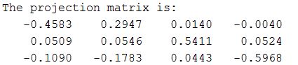
The total residual is: <0.0445>
In compute_camera_center() I use the projection Matrix and then compute the camera center as shown in the code below:
	Q = M(:,1:3);
	m4 = M(:,4);
	Q_inv = inv(Q);
	Center = -mtimes(Q_inv,m4);
Result
The estimated location of camera is: <-1.5127, -2.3517, 0.2826>
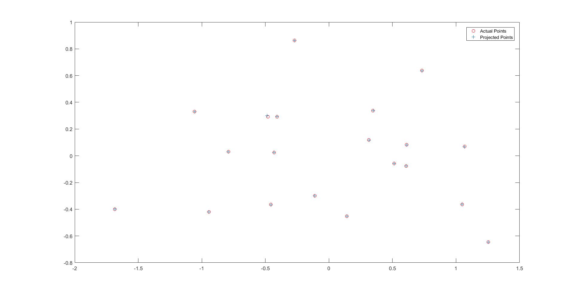
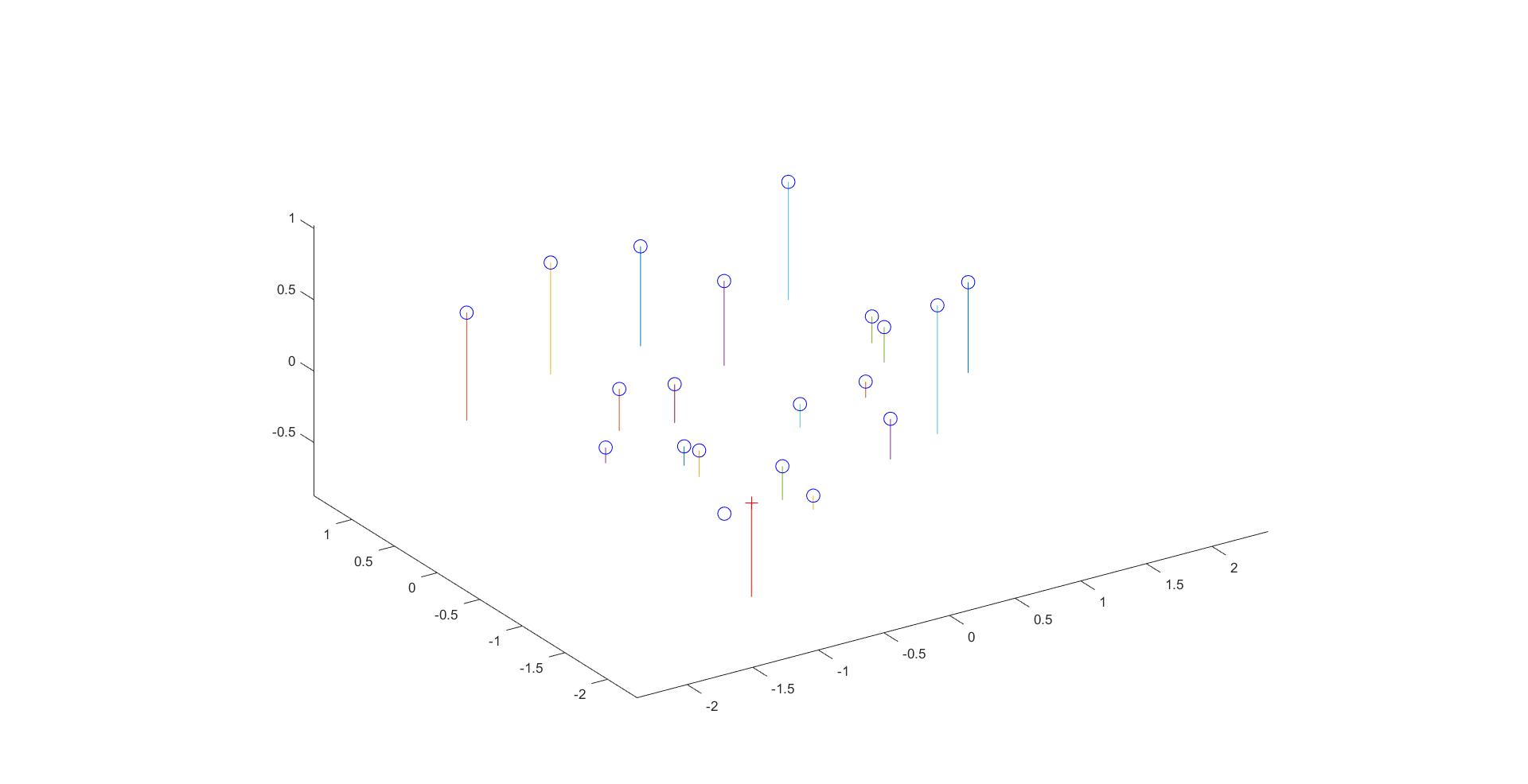
The graph for actual points vs projected points
The estimated 3D location of the camera
Fundamental Matrix Estimation and Normalization
In estimate_fundamental_matrix(), in the implementation without normalization, I intially create an array given the two 2D arrays and then compute the svd of this matrix. And then reshaping this matrix to [3 3] and then set the smallest value to 0 hence making the rank of the matrix 2. And then I return the 3x3 Fundamental Matrix
The code for generating the Fundamental matrix
	A = ones(m,9);
	for i = 1 : m
		A(i,1:2) = Points_b(i,1) * Points_a(i,1:2);
		A(i,3) = Points_b(i,1);
		A(i,4:5) = Points_b(i,2) * Points_a(i,1:2);
		A(i,6) = Points_b(i,2);
		A(i,7:8) = Points_a(i,1:2);
	end
	[~,~,V] = svd(A);
	f = V(:,end);
	F = reshape(f,[3 3])';
	[U,S,V] = svd(F);
	S(3,3) = 0;
	F_matrix = U*S*V';
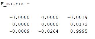
Result
The Fundamental Matrix that I obtain without normalization:
Fundamental Matrix Normalization
In estimate_fundamental_matrix(), in the implementation with normalization, I intially normalize the given two 2D arrays as shown in the code below and then I use the transformation matrices to get the fundamental matrix back.
The code for generating the normalized points
	[m,~] = size(Points_a);
	mean_a = mean(Points_a);
	mean_b = mean(Points_b);
	std_a = std2(bsxfun(@minus,Points_a,mean_a));
	std_b = std2(bsxfun(@minus,Points_b,mean_b));
	S_matrix_a =  [1.0/std_a 0 0; 0 1.0/std_a 0; 0 0 1];
	S_matrix_b =  [1.0/std_b 0 0; 0 1.0/std_b 0; 0 0 1];
	M_matrix_a = [1 0 -mean_a(1,1); 0 1 -mean_a(1,2); 0 0 1];
	M_matrix_b = [1 0 -mean_b(1,1); 0 1 -mean_b(1,2); 0 0 1];
	Points_a_temp = horzcat(Points_a,ones(m,1));
	Points_b_temp = horzcat(Points_b,ones(m,1));
	Points_a_norm = mtimes(mtimes(S_matrix_a,M_matrix_a),Points_a_temp')';'
	Points_b_norm = mtimes(mtimes(S_matrix_b,M_matrix_b),Points_b_temp')';'
	T_a = mtimes(S_matrix_a, M_matrix_a);
	T_b = mtimes(S_matrix_b, M_matrix_b);

	%Transformating back
	F_matrix = mtimes(mtimes(T_b',F_matrix_temp),T_a);
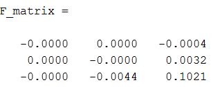
Result
The Fundamental Matrix that I obtain after normalization:
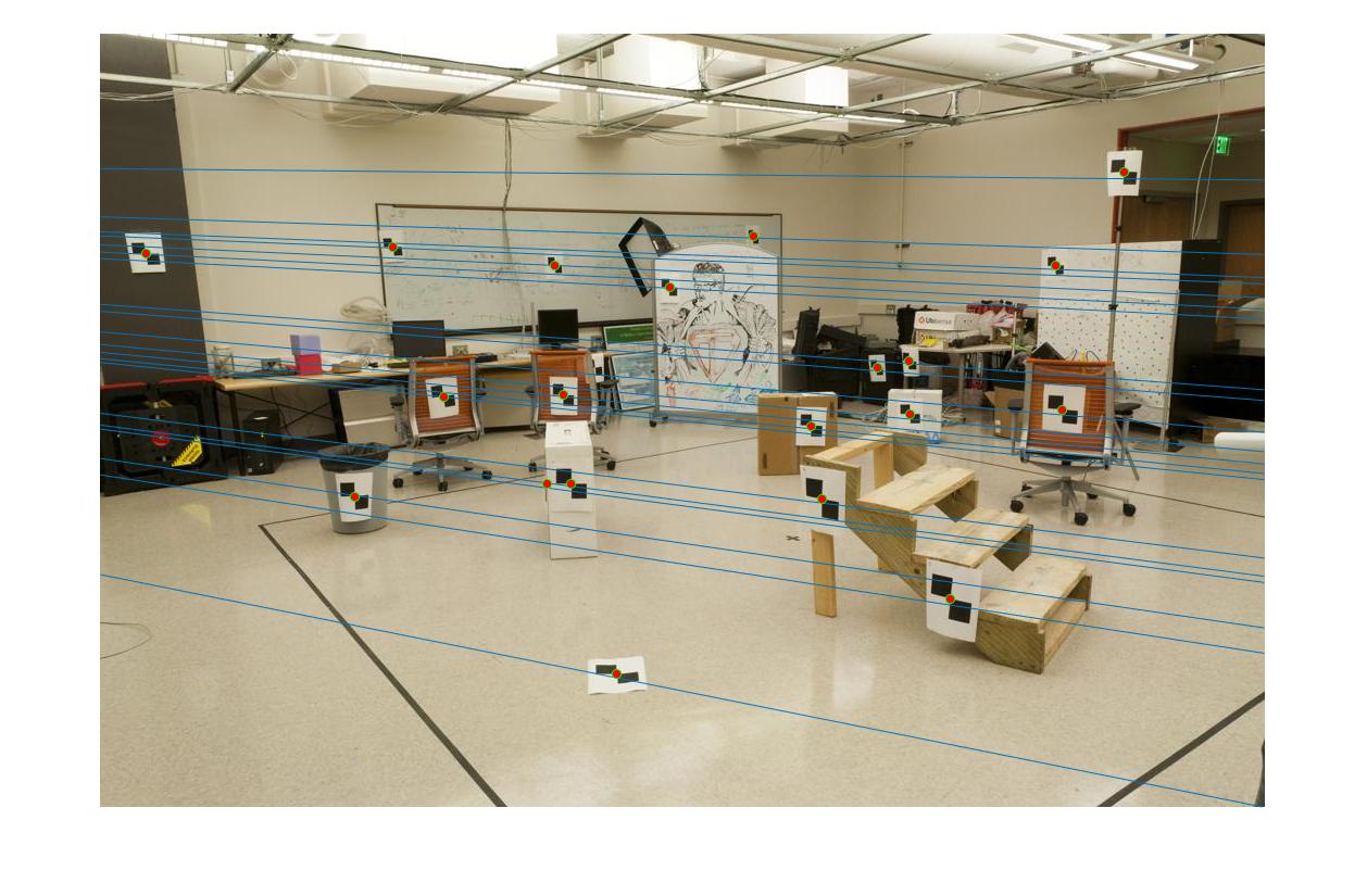
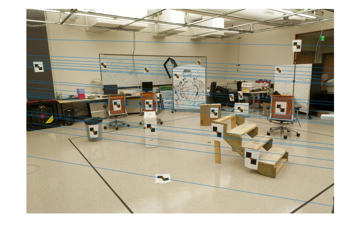
The epipolar lines for the two images:
|

|
The two images on the top are the images obtained without normalization, while the bottom images are the ones obtained after normalization.
It is evident from the images that normalization helps in getting a better result as the epipolar lines pass right through the centres in the bottom two images, while they are slightly off in the top two images.
Fundamental Matrix with RANSAC
In ransac_fundamental_matrix(), I start by sampling a small number of points from the dataset. I have sampled 8 datapoints in my code. Then based on these 8 samples I find a fundamental matrix by calling the above method. Once I get the fundamental matrix I compute xFx' for every pair (x,x') given in the dataset. I have vectorized this operation. Let's call this V
Inliers are points whose absolute value obtained above i.e. |V| is less than a preset threshold value. I tried different values and 0.001 to 0.005 worked well for me, with 0.005 giving the highest number of inliers and good results. I count the number of inliers thus obtained with the maximum inliers I have and if they are more than the current max, I store this fundamental matrix as the best one. I repeat this for 2000 iterations before finding the best fundamental matrix
Once I have this best fundamental matrix, I back calculate the inliers, using the max_inliers I have and then use these indices to get the inliers from the given dataset. And then I return top 30 of these inlers, where the values are sorted
The code for RANSAC
	iterations = 2000;
	points_to_subsample = 8;
	threshold = 0.0009;
	top_n = 30;
	[m,~] = size(matches_a);
	Points_a_temp = horzcat(matches_a,ones(m,1));
	Points_b_temp = horzcat(matches_b,ones(m,1));
	max_inliers = 0;
	B_F_matrix = zeros(3,3);
	for i = 1 : iterations
		disp(i)
		rows = randsample(m,points_to_subsample);
		F_matrix = estimate_fundamental_matrix(matches_a(rows,:), matches_b(rows,:));
		prod_temp = mtimes(mtimes(Points_b_temp,F_matrix),Points_a_temp');
		prod = diag(prod_temp);
		liers = abs(prod) < threshold;
		inliers = find(~liers);
		if size(inliers,1) > max_inliers
			B_F_matrix = F_matrix;
			max_inliers = size(inliers,1);
		end
	end
	prod_temp = mtimes(mtimes(Points_b_temp,B_F_matrix),Points_a_temp');
	prod = abs(diag(prod_temp));
	[~,indices] = sort(prod);
	max_indices = indices(1:max_inliers);
	disp(max_inliers)
	if top_n < size(max_indices,1)
		cap = top_n;
	else
		cap = size(max_indices,1);
	end
	indices_to_take = max_indices(1:cap);
	inliers_a = matches_a(indices_to_take,:);
	inliers_b = matches_b(indices_to_take,:);
	Best_Fmatrix = B_F_matrix;
Result
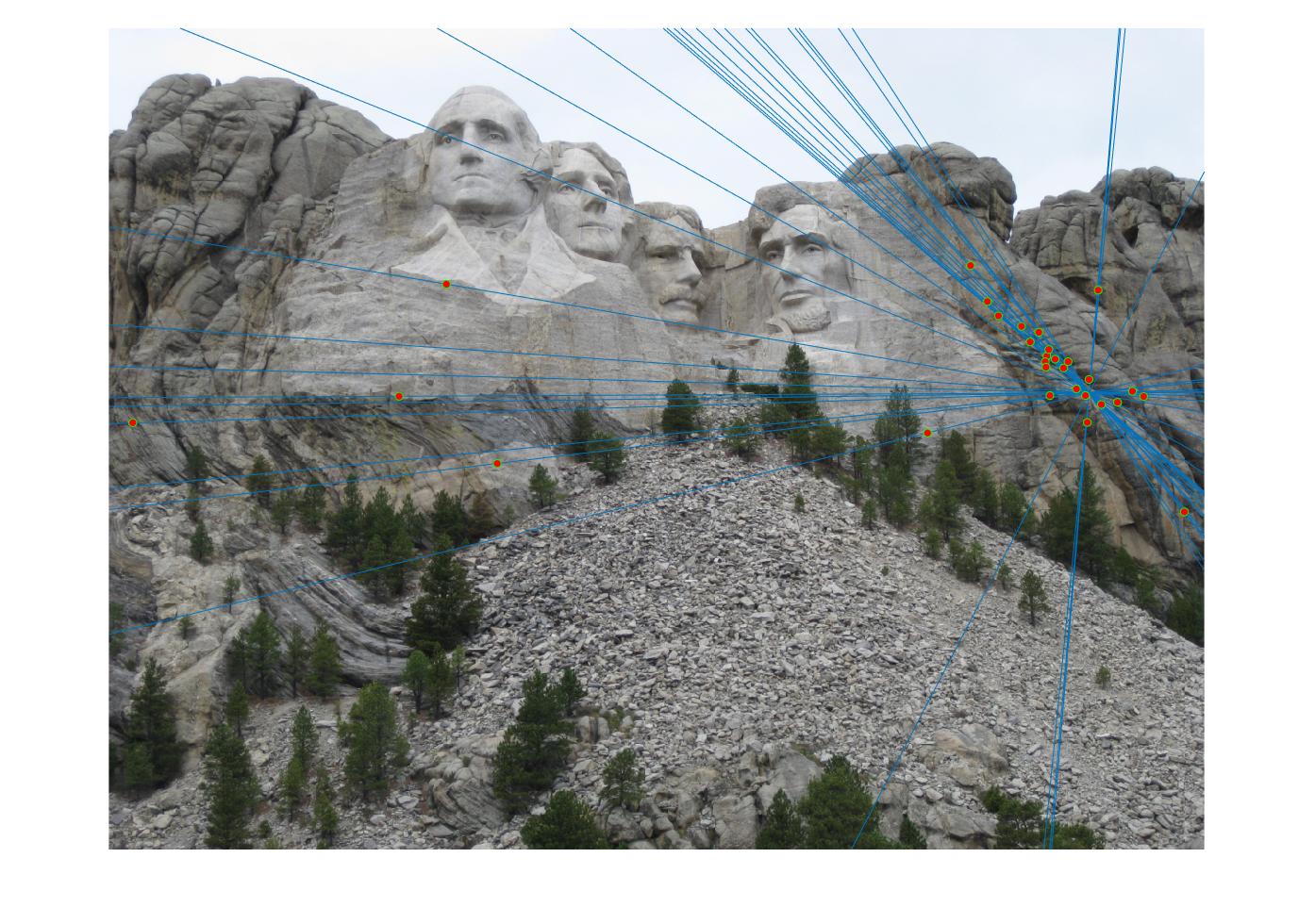
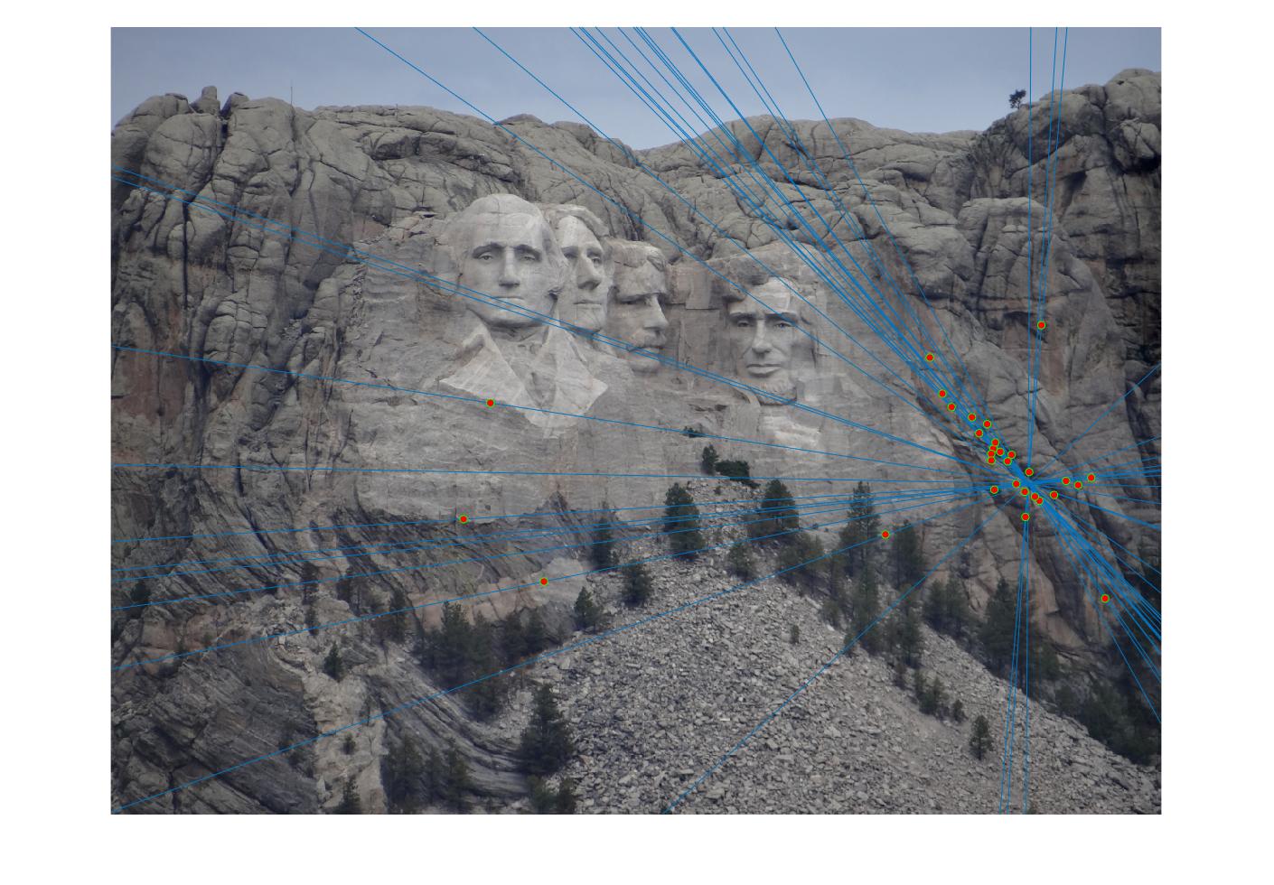
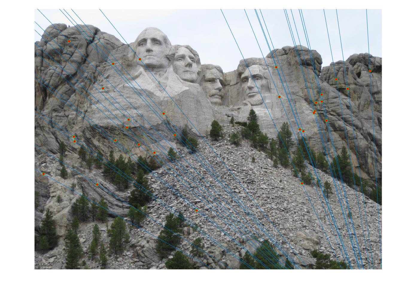
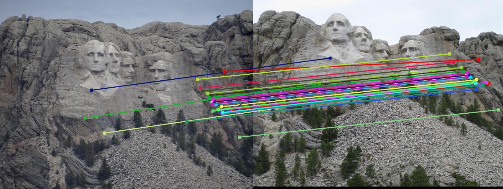
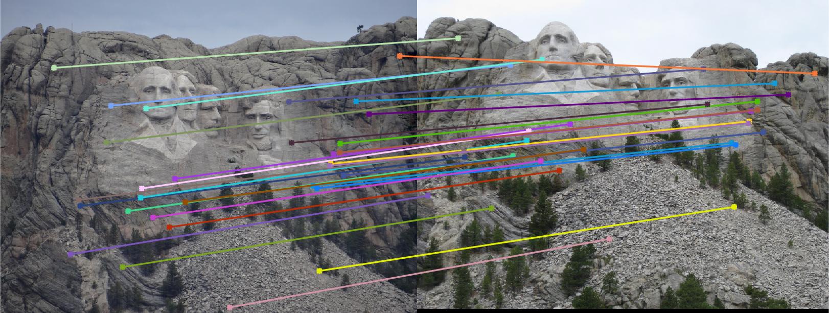
The result I get after applying the above algorithm to a set of images
First row is epipolar lines without normalization
Second row is epipolar lines with normalization
Third row is matching without normalization
Fourth row is matching with normalization
Mount Rushmore
|
|
|
|
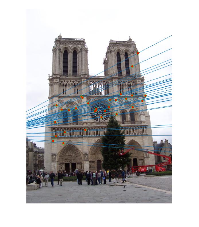
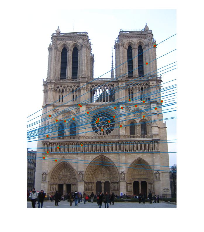
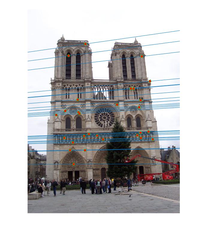
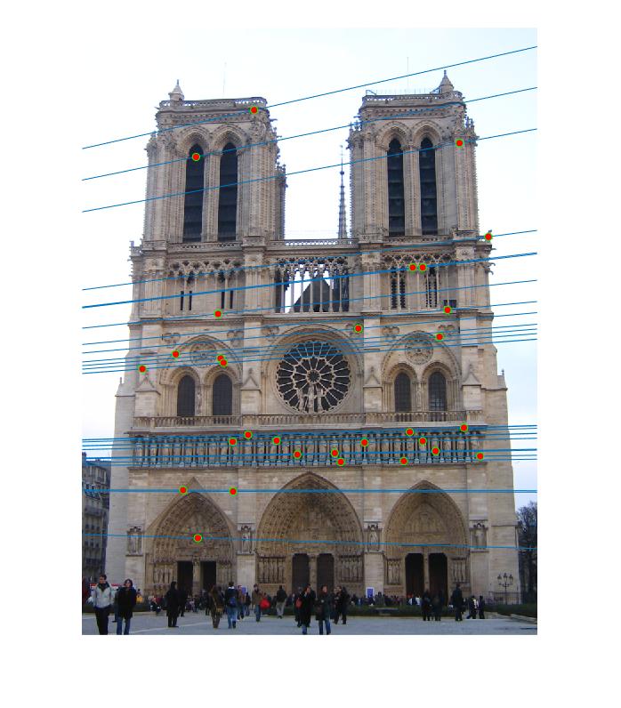
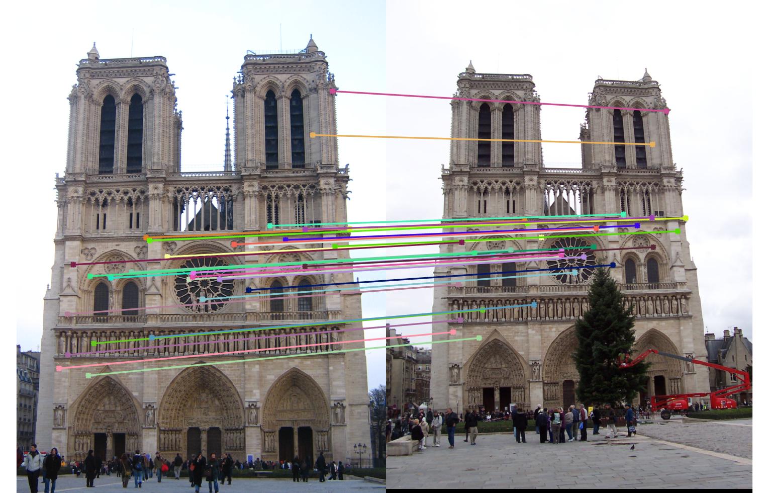
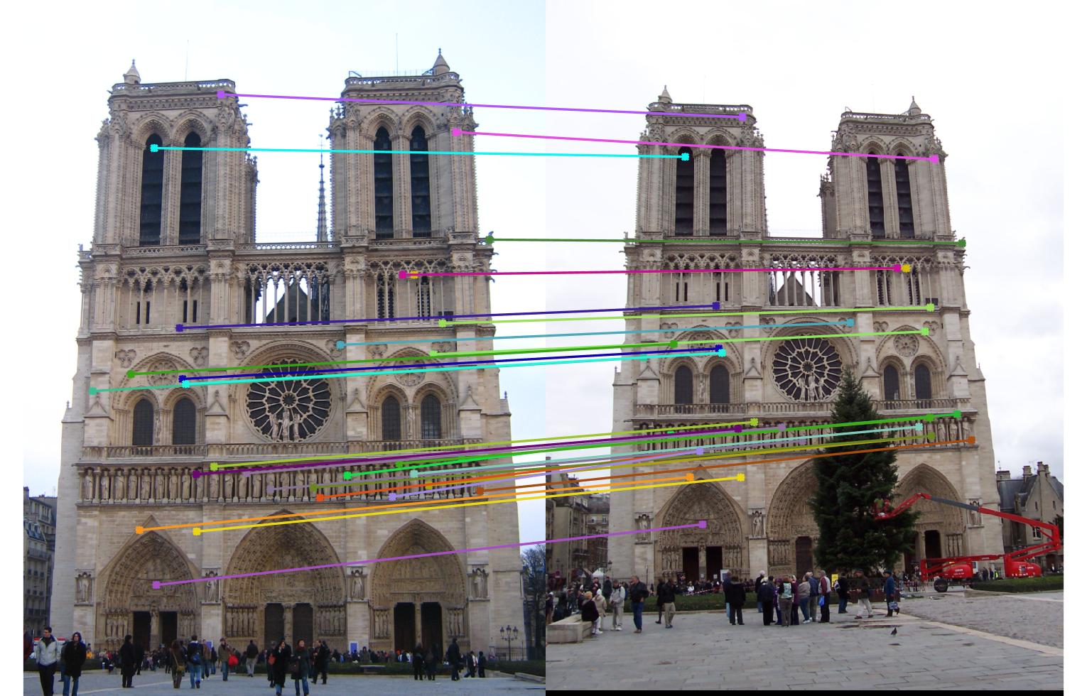
Notre Dame
First row is epipolar lines without normalization
Second row is epipolar lines with normalization
Third row is matching without normalization
Fourth row is matching with normalization
|
|
|
|
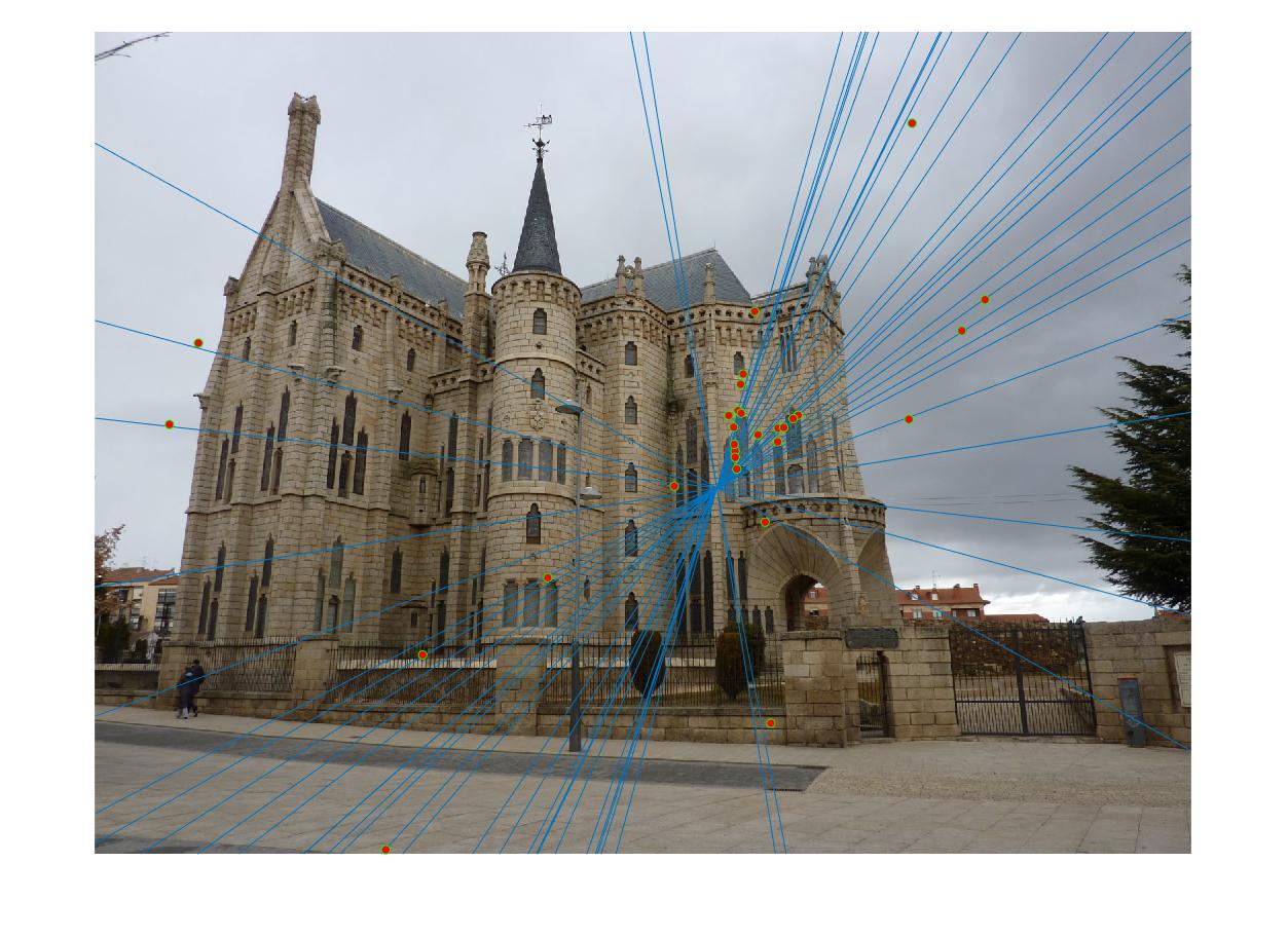
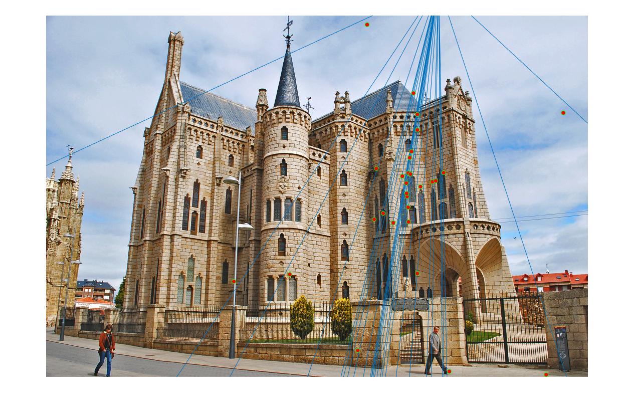
Episcopal Gaudi
First row is epipolar lines without normalization
Second row is epipolar lines with normalization
Third row is matching without normalization
Fourth row is matching with normalization
|
|
|
|
|
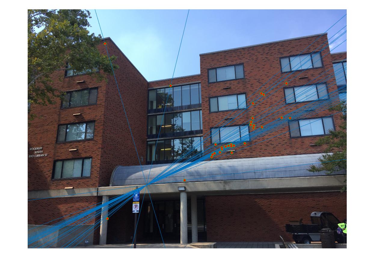
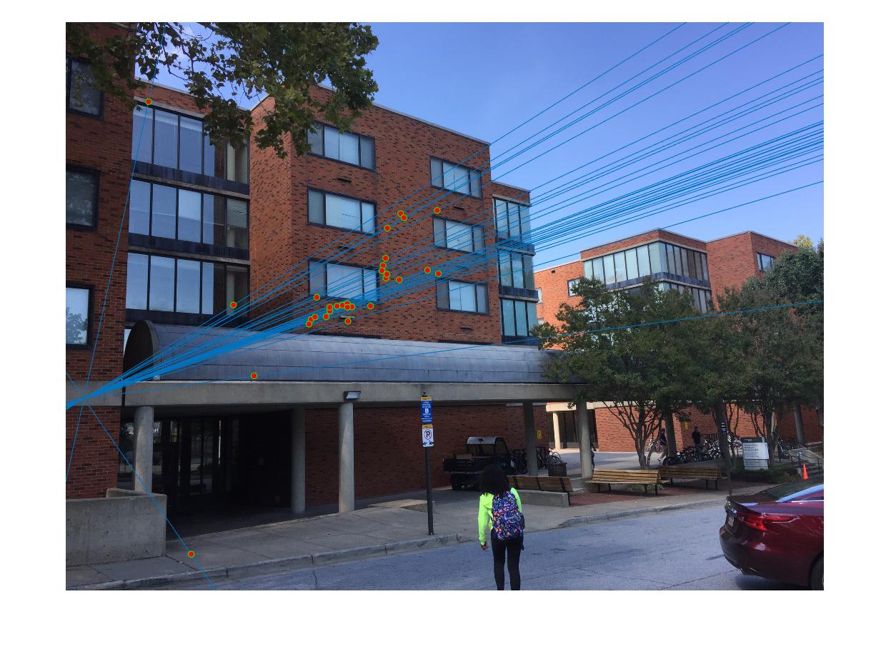
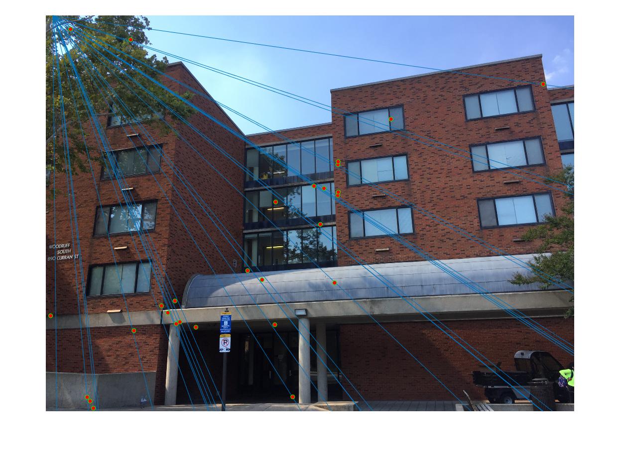
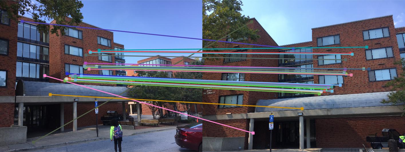
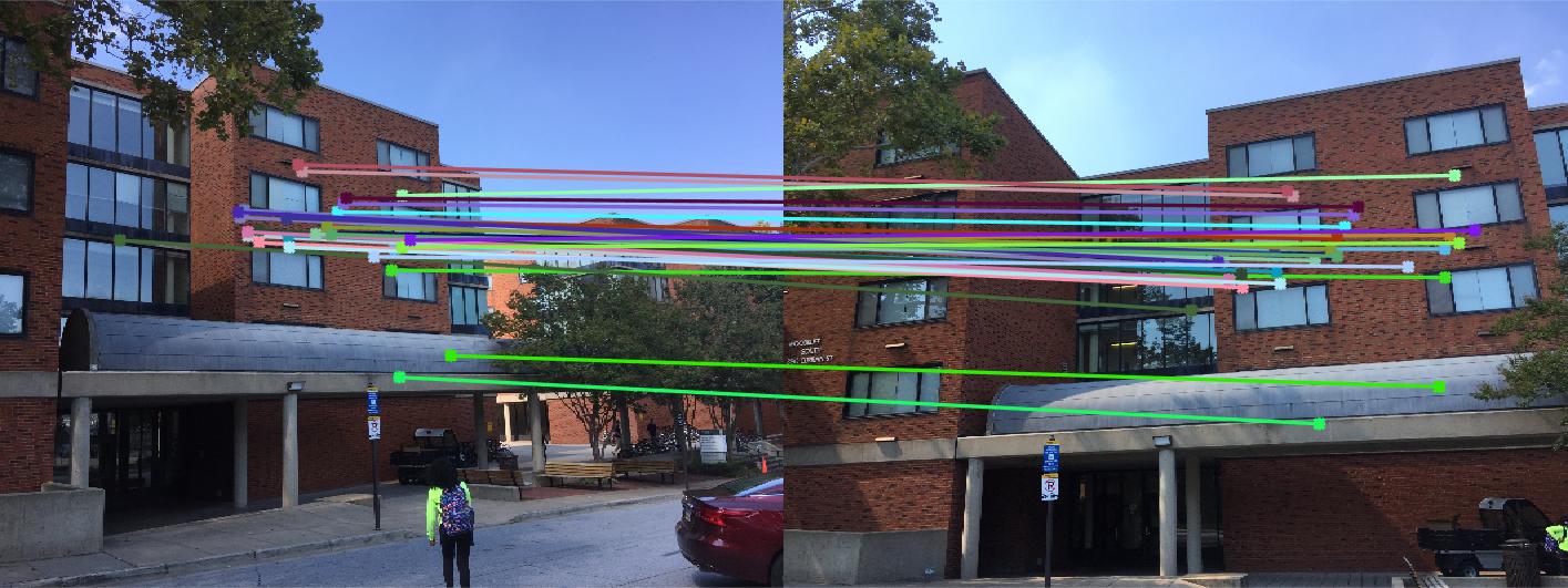
Woodruff Dorm
First row is epipolar lines without normalization
Second row is epipolar lines with normalization
Third row is matching without normalization
Fourth row is matching with normalization
|

|
|
|
The most significant difference in results with and without normalization is observed in Episcopal Gaudi Images.
I replot the images to point out the difference. The left column shows the results without normalization while the right columns show the effect of normalization on the same set of images.
|
|
|
|
|
|