Steven Calhoun

Part 1: Camera Calibration

To solve for the projection matrix we need to set up a homogenous set of equations using the 3D world points and 2D image points. This matrix is equivelant to K[R|T]. Where K is the intrinsic matrix, R is the rotation of the matix, and T is the translation of the camera. The system to solve for the projection matrix is set up like so:

                                                    [M11   [u1
                                                     M12    v1
   [X1 Y1 Z1 1 0  0  0  0 -u1*X1 -u1*Y1 -u1*Z1       M13    .
    0  0  0  0 X1 Y1 Z1 1 -v1*Z1 -v1*Y1 -v1*Z1       M14    .
    .  .  .  . .  .  .  .    .     .      .          M21    .
    .  .  .  . .  .  .  .    .     .      .      *   M22 =  .
    .  .  .  . .  .  .  .    .     .      .          M23    .
    Xn Yn Zn 1 0  0  0  0 -un*Xn -un*Yn -un*Zn       M24    .
    0  0  0  0 Xn Yn Zn 1 -vn*Zn -vn*Yn -vn*Zn]      M31    .
                                                     M32    un
                                                     M33    vn]
        

In this X, Y, Z are the coordinates of a 3D point and u and v are the coordinates of a 2D image point. We can set this matrix up using the points passed to the function then solve the system using MATLAB's SVD function. Taking the V matrix from the solution and reshaping it gives us the projection matrix.

    % Calculate M with svd
    [U, S, V] = svd(A);
    M = V(:,end);
    M = reshape(M,[],3)';
        

This allows us to map 2D image points to 3d world points. We can also access the different elements of the projection matrix. For this part of the project we want to extract the intrinsic matrix so that we can recover the camera's center. The intrinisc matrix is of the form

   [ α  s  u0
     0  β  v0
     0  0  1 ]
        

To recover the camera center we can simply compute -Q-1m4

    Q = M(:, 1:3);
    m4 = M(:, 4);
    Center = -inv(Q)*m4;
        

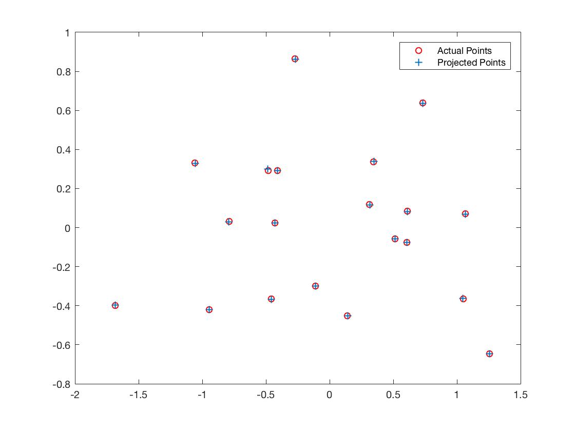
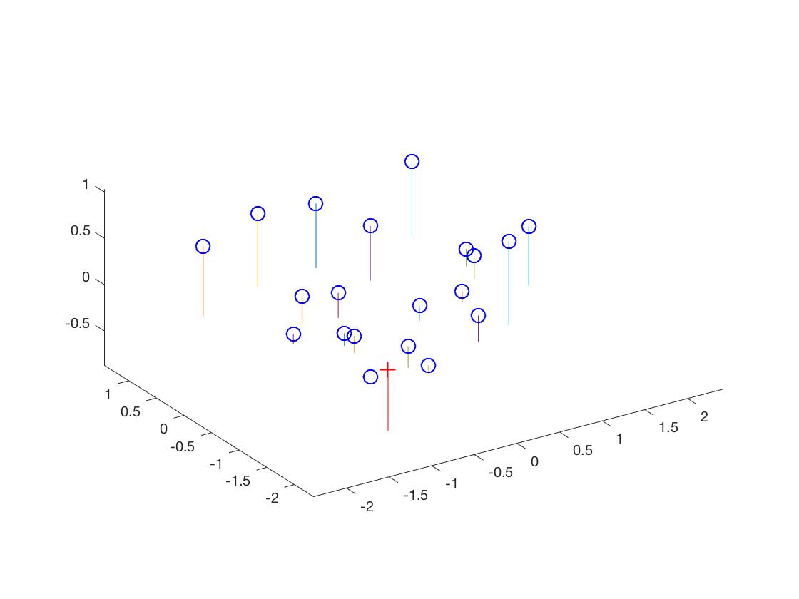
In part 1 I achieved a total residual of 0.0445, computed a camera center of <-1.5127, -2.3517, 0.2826>, and computed a projection matrix of

     -0.4583    0.2947    0.0140   -0.0040
      0.0509    0.0546    0.5411    0.0524
     -0.1090   -0.1783    0.0443   -0.5968
        

For the unnormalized points I achieved a total residual of 15.545, computed a camera center of <303.1000, 307.1843, 30.4217>, and computed a projection matrix of

    -0.0069    0.0040    0.0013    0.8267
    -0.0015   -0.0010    0.0073    0.5625
    -0.0000   -0.0000    0.0000    0.0034
        

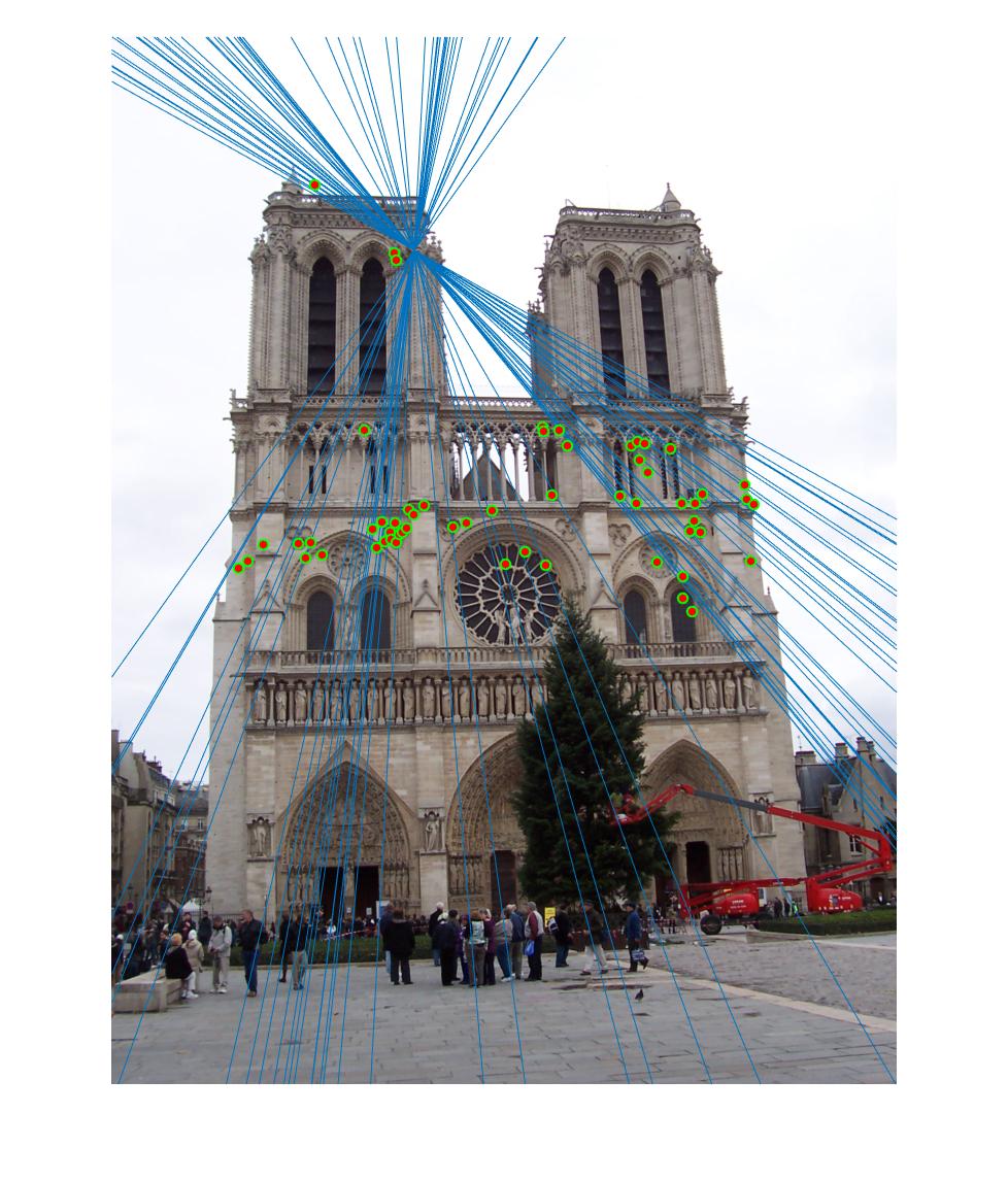
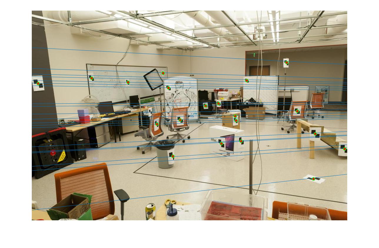
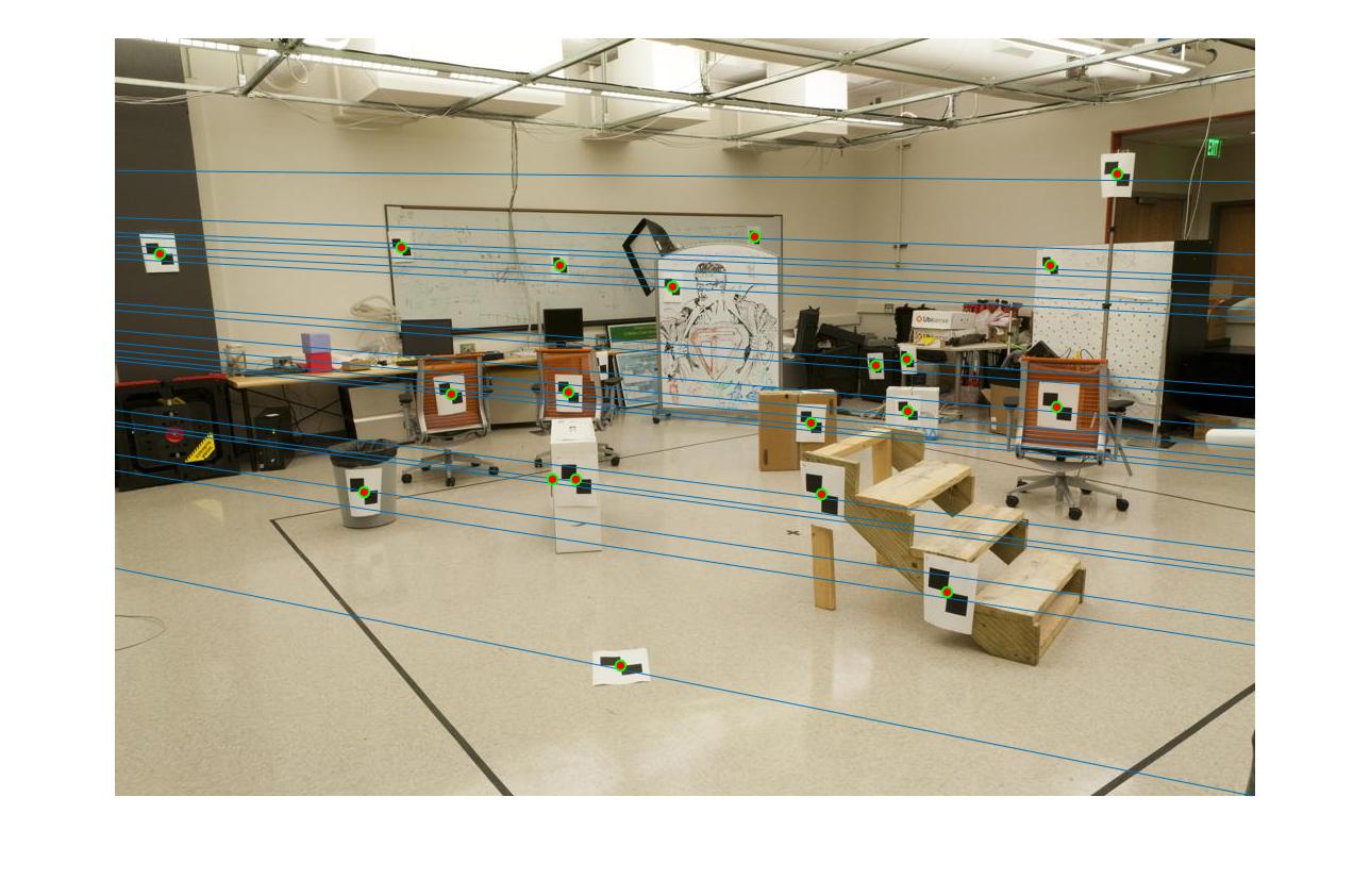
Part 2: Fundamental Matrix Estimation

In this part we calculate the fundamental matrix, which maps points in one image to lines in another. This requires setting up a matrix similar to the one in the previous part. We use the 8-point algorithm to do solve the matrix. We first setup the matrix using the passed 2D image correspondences. The matrix is set up as:

    [u'*u u'*v u' v'*u v'*v v' u v 1]
        

The matrix A has n rows one for each correspondence passed to the function. Once this matrix is set up we can solve Af=0 using MATLAB's SVD function. After that we need to enforce the singularity constraint. We can also do this with SVD.

    [U, S, V] = svd(A);
    f = V(:, end);
    F_norm = reshape(f, [3,3])';

    [U, S, V] = svd(F_norm);
    S(3,3) = 0;
    F_norm = U*S*V';
        

This algorithm is designed be to used with 8 correspondences, but if all the correspondences are perfect like the ground truth points, then more can be used. An initial step to my implementation of this algorithm is to normalize the points. This involves ensuring the average distance to the centroid of all the points is the square root of 2. We can then create a linear transform to scale and shift all of the points

              [s 0 0] [1 0 -cu] [u]
(u', v', 1) = [0 s 0] [0 1 -cv] [v]
              [0 0 1] [0 0  1 ] [1]
        

This linear transform let's us normalize all of the corresponding points in each image. After estimating the fundamental matrix we can then denormalize it using F = bTFaT. Where b^T and a^T are the linear transforms for image A and image B.

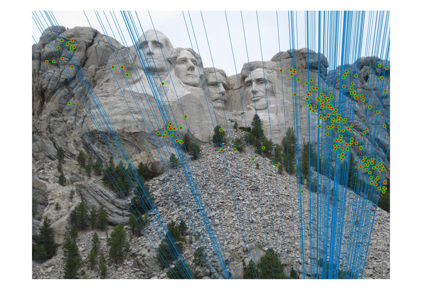
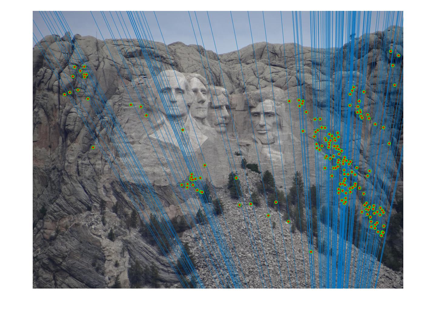
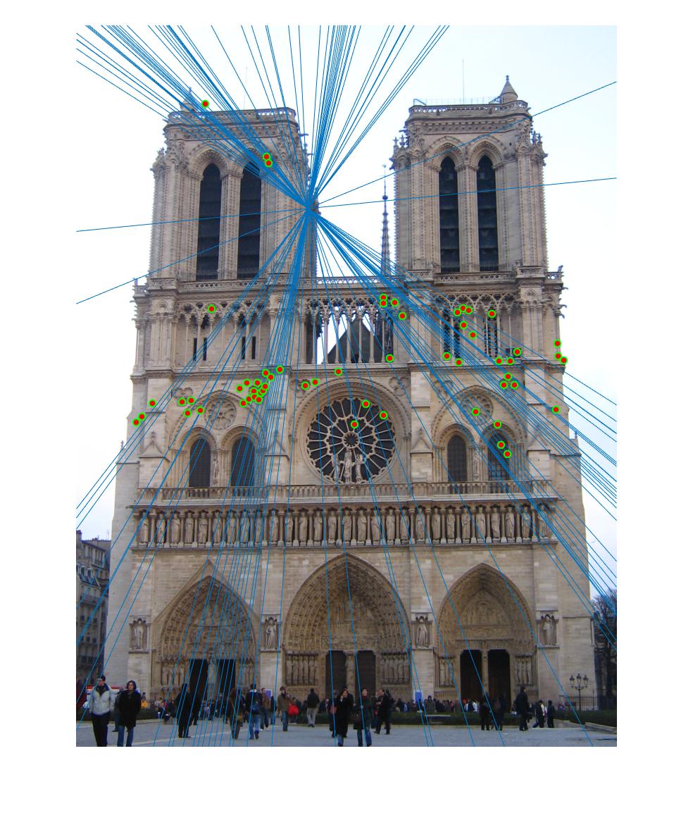
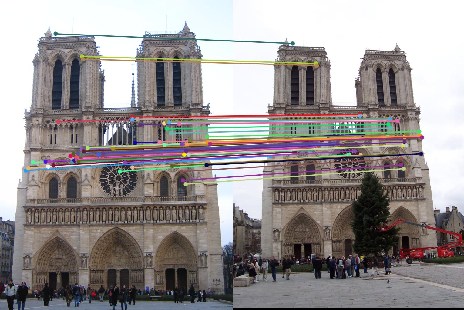
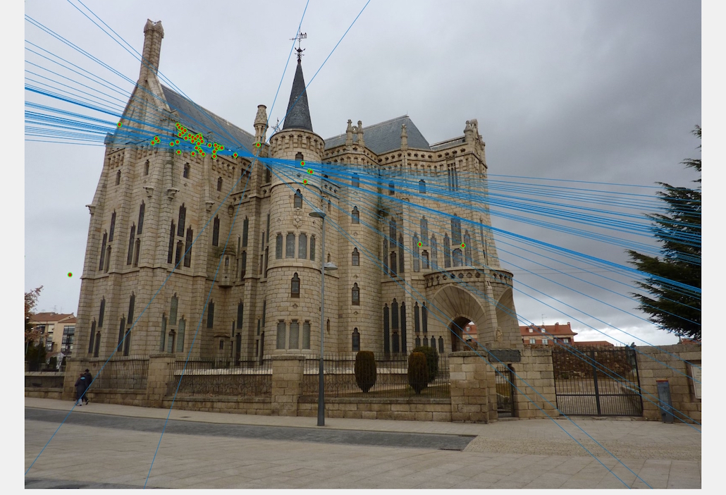
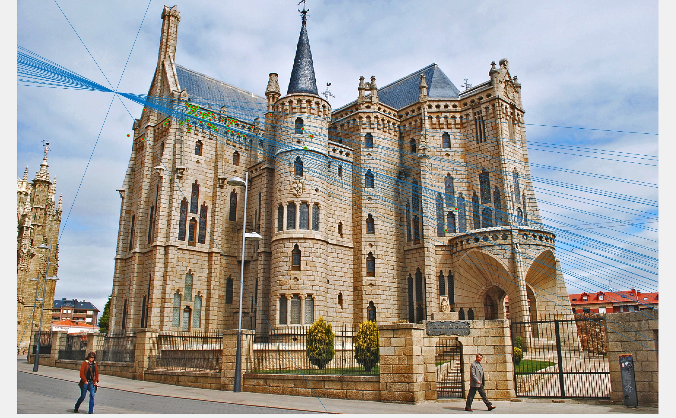
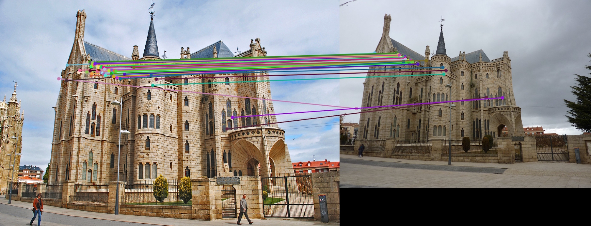
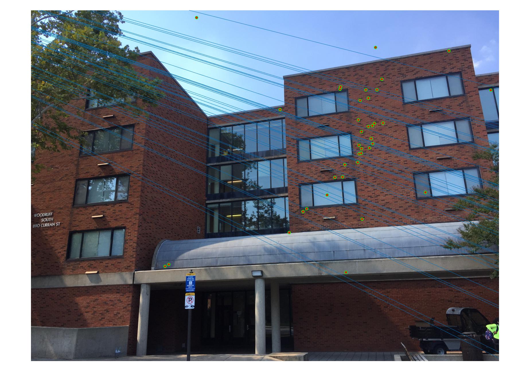
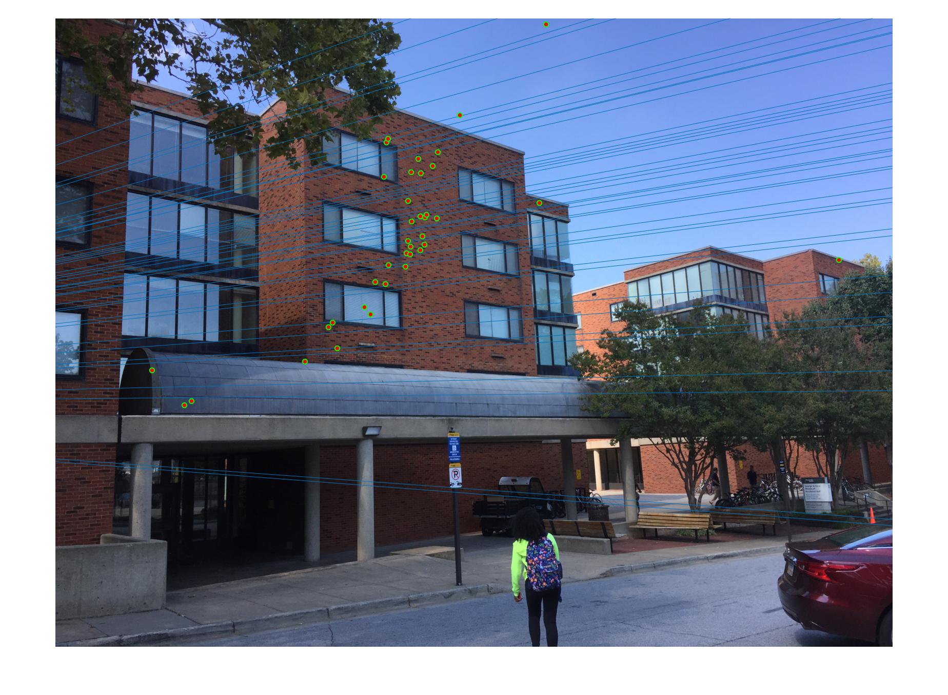
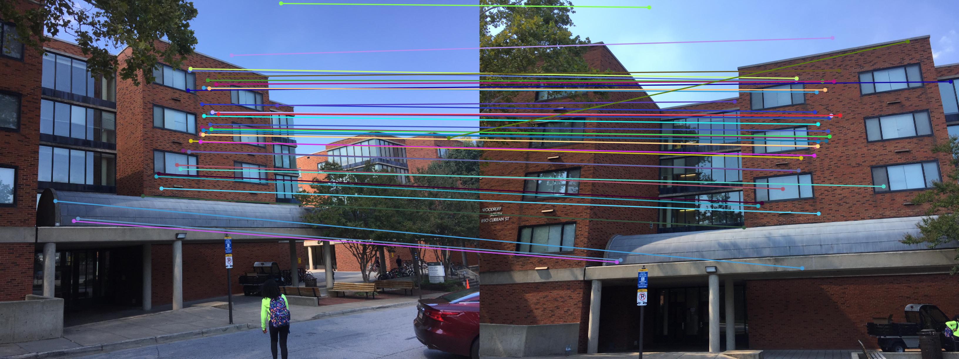
Part 3: RANSAC Fundamental Matrix

The final part was to attempt to estimate the fundamental matrix of two images using correspondances produced by a SIFT function instead of ground truth points. It is much more likely that these points are not as good as the ground truth points and given 8 points we may not calculate a very good fundamental matrix. To help solve this we use RANSAC. Given a list of correspondances we will:

1. Choose 8 random correspondances
2. Estimate the fundamental matrix with these points
3. Count the number of inliers with this fundamental matrix

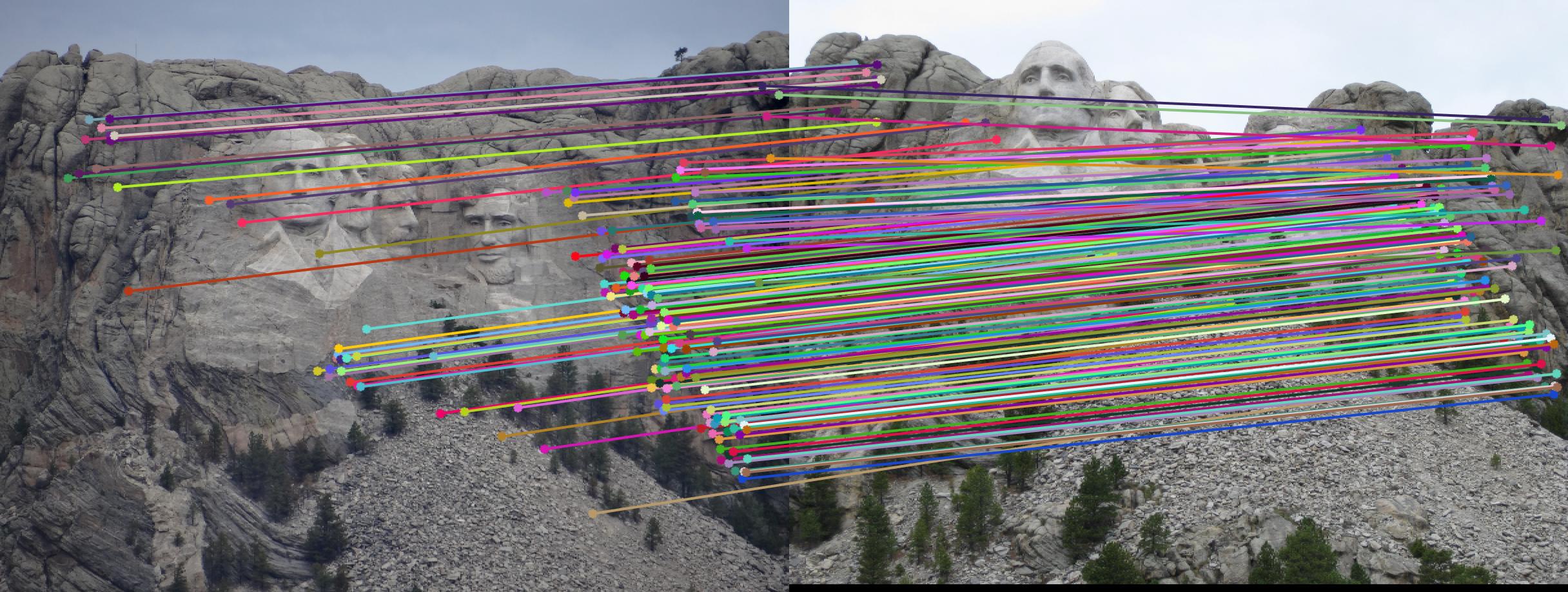
This process will be repeated N times and the fundamental matrix with the largest number of inliers will be returned. We can choose N by specificying

• p: the chance of success
• e: the probability of outliers
• s: the number of points to be sampled

N can then be calculated using N = log(1-p)/log(1-(1-e)s);. We also must choose a sigma, the theshold between an inlier and outlier. Once a fundamental matrix has be estimated we use xTFx' to determine if the correspondenc is an inlier or outlier. For a perfect match, this evaluates to zero, but if the value is below the threshold then it is considered an inlier.