Project 3 / Camera Calibration and Fundamental Matrix Estimation with RANSAC
In this project, we look at the problem of camera calibration through the following three steps:
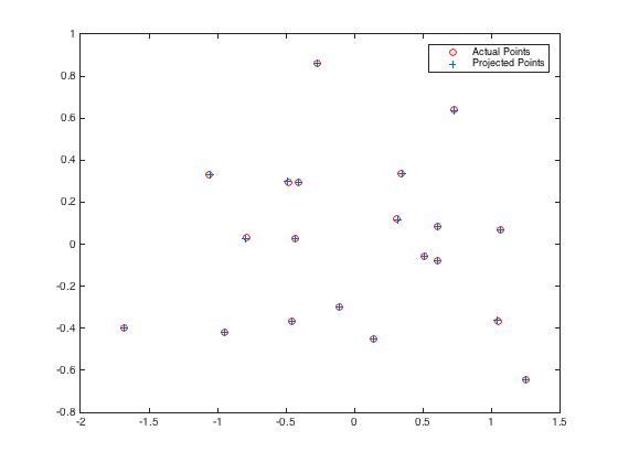
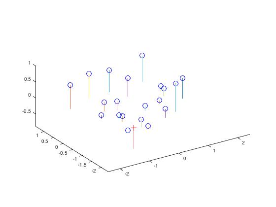
- Calculate the projection matrix from the given 2D and 3D points as well as the camera center.
- Calculate the fundamental matrix from the given set of corresponding 2D points.
- Estimate the fundamental matrix from noisy data (matched points with SIFT) using RANSAC to deal with the noisy data.
Projection Matrix & Camera Center
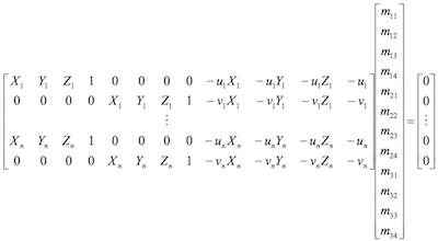
In this part of the project, I calculate the projection matrix by building the following homogeneous linear system:
0.4583   -0.2947   -0.0140    0.0040
-0.0509   -0.0546   -0.5411   -0.0524
0.1090    0.1783   -0.0443    0.5968
<-1.5127, -2.3517, 0.2826>
|
Fundamental Matrix
Then, I calculate the fundamental matrix with the following equation:
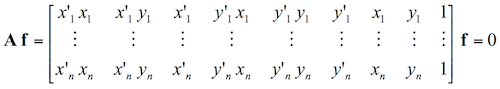
-6.60698417012863e-07	8.82396296136248e-06	-0.000907382302152503
7.91031620841439e-06	1.21382933020618e-06	-0.0264234649901806
-0.00188600197690852	0.0172332901072652	0.999500091906723
-5.36264198382353e-07	8.83539184115726e-06	-0.000907382264407744
7.90364770858056e-06	1.21321685010730e-06	-0.0264234649922034
-0.00188600204023565	0.0172332901014488	0.999500091906703
|
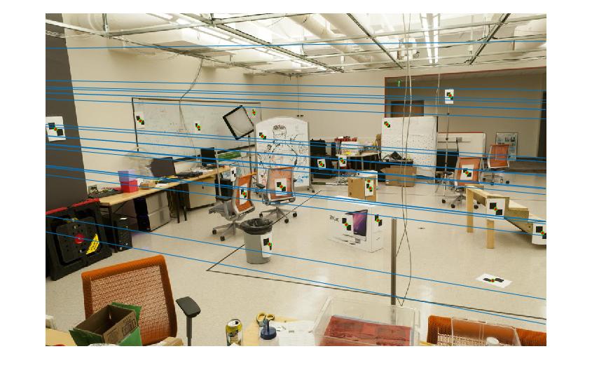
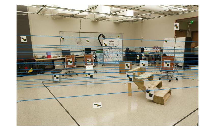
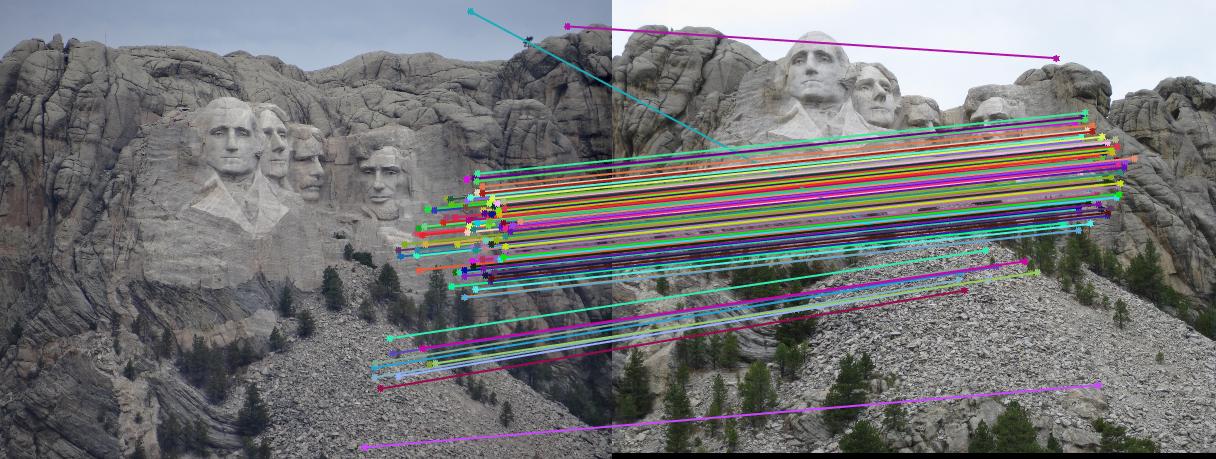
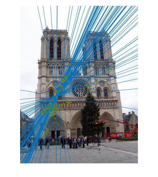
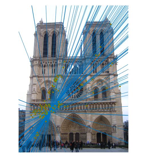
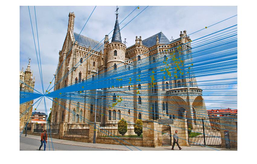
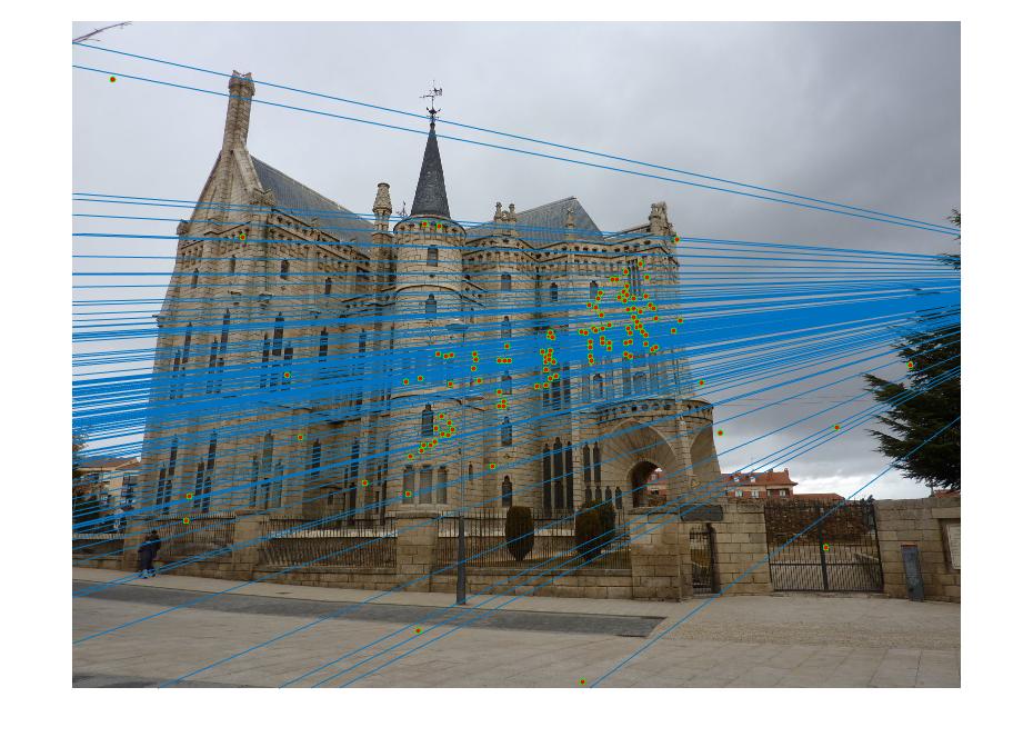
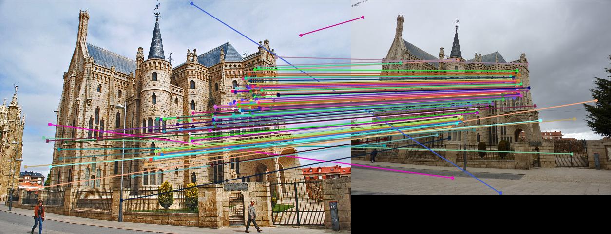
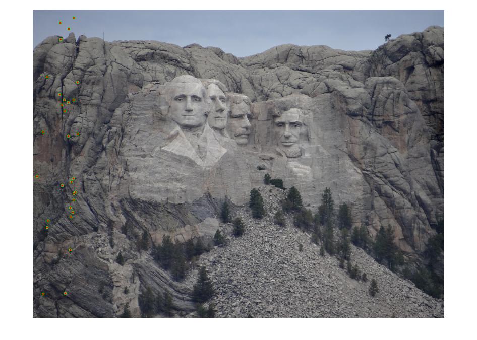
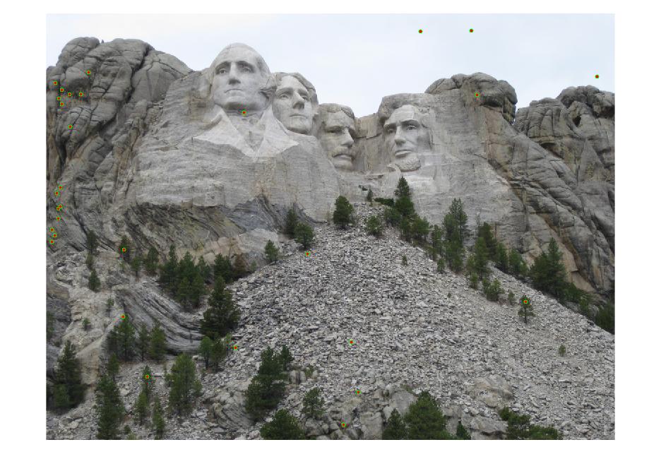
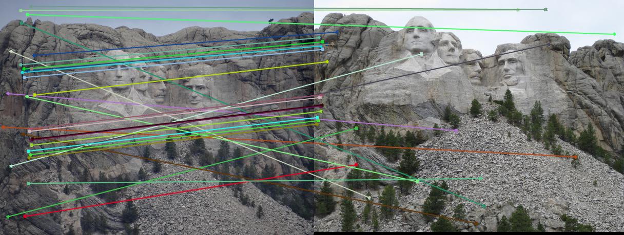
Fundamental Matrix & RANSAC
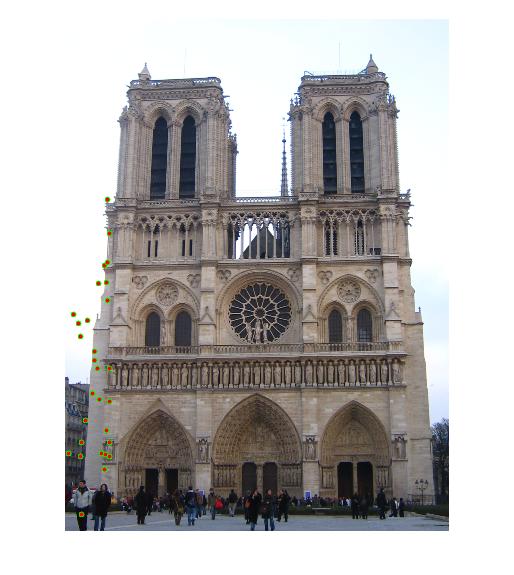
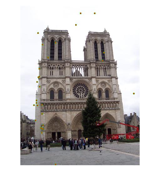
First, the VL Feat implementation of SIFT is used to produce descriptors and possible matches.
| Image | SIFT Descriptors in Image A | SIFT Descriptors in Image B | Possible Feature Matches | Inlier Feature Matches |
|---|---|---|---|---|
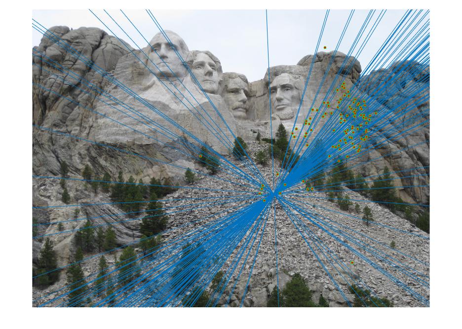
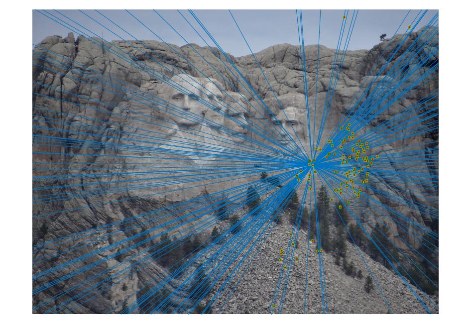
| Rushmore | 5581 | 5246 | 825 | 87 |
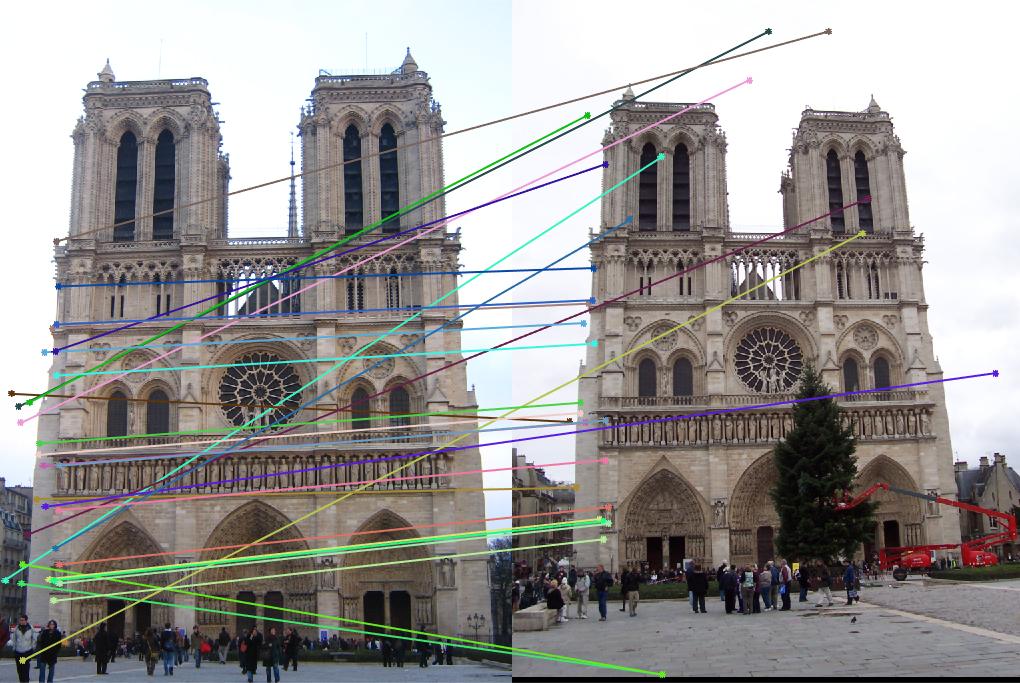
| Notre Dame | 3396 | 3025 | 851 | 96 |
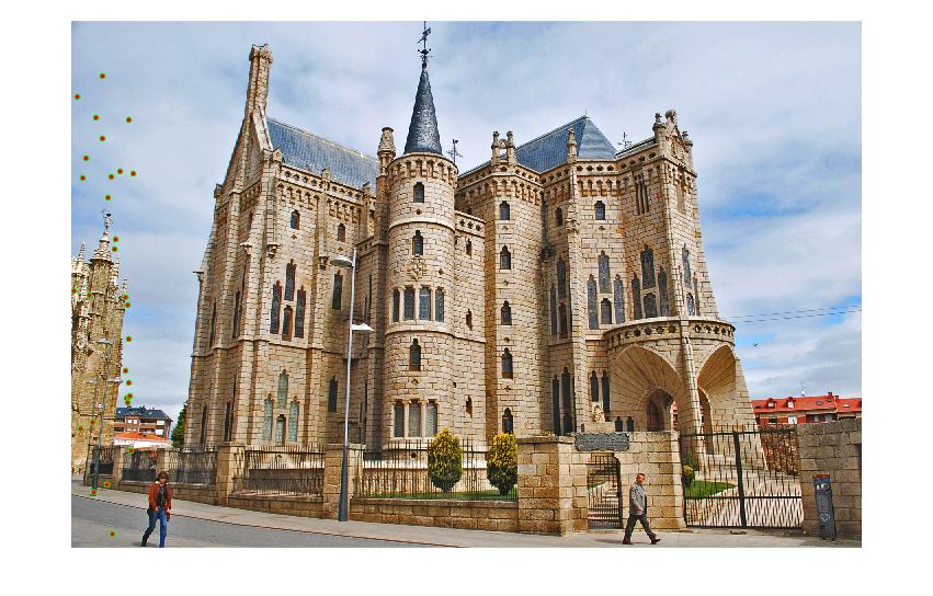
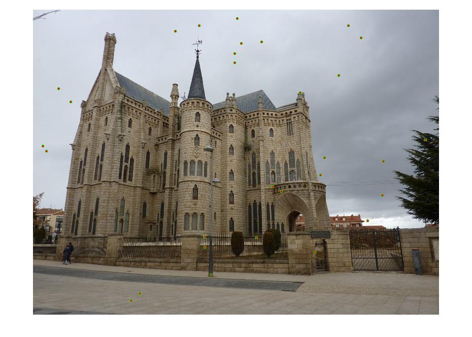
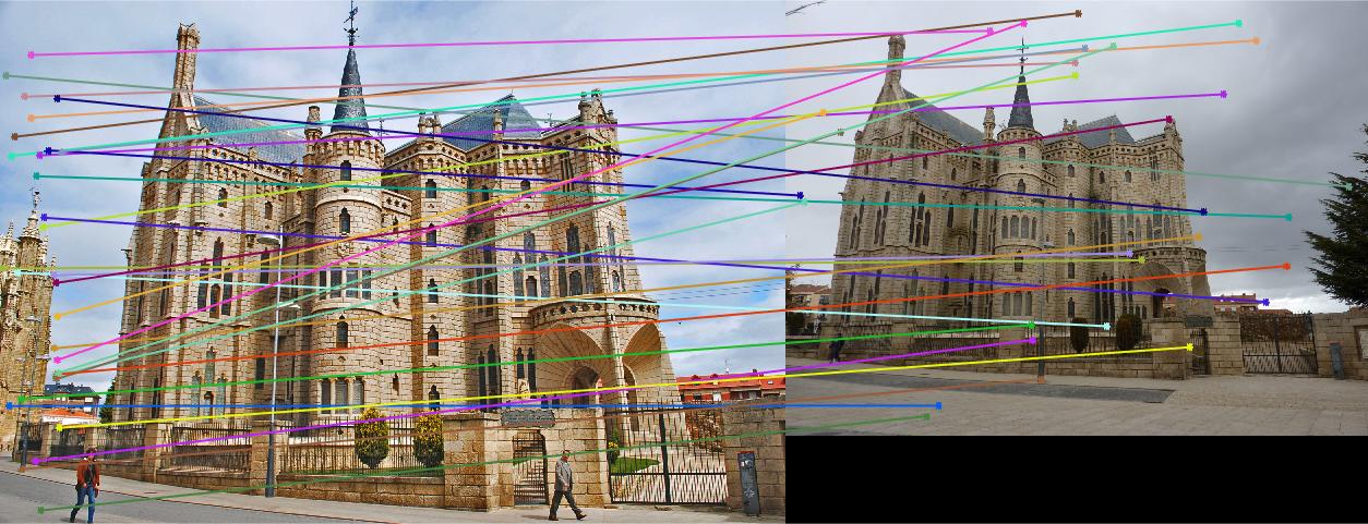
| Gaudi | 12683 | 8766 | 1062 | 124 |
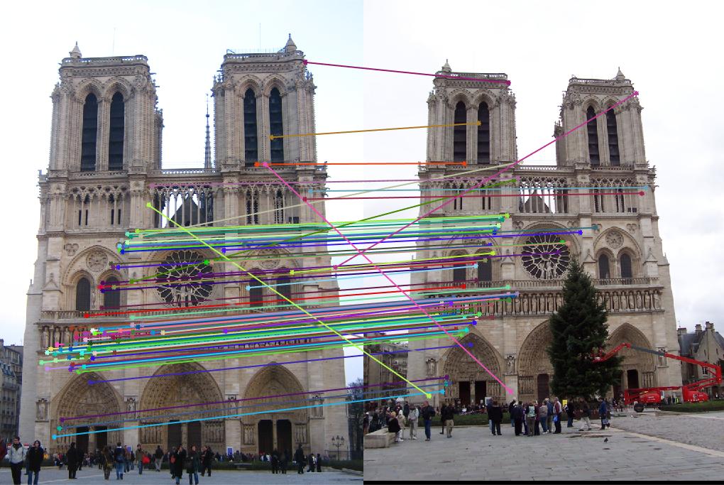
Results
|
|
|
Graduate Portion
In this portion of the assignment, I improve the above results with normalization. As mentioned in the lecture, the numbers can easily blow up, with certain regions of the matrix holding values much larger than other sections. To correct for this, I scale these coordinates by computing the scale factor from the mean coordinates. I tried two methods of scaling. The first was to use the maximum value from the points to scale, which led to a difference between the original fundamental matrix and the normalize fundamental matrix, the difference of which you can see here at each index for the Rushmore image pair:
-0.0000    0.0000   -0.0000
 0.0000    0.0000   -0.0009
-0.0003   -0.0007    0.5667
-0.0000    0.0000   -0.0081
-0.0000   -0.0000    0.0150
 0.0047   -0.0196    1.6878
Results with Normalization
|
|
|