Project 3 / Camera Calibration and Fundamental Matrix Estimation with RANSAC
The project is divided into three parts as listed below.
- Determining projection matrix and camera center
- Determining fundamental matrix for two images using least square regression
- Determining optimal fundamental matrix using RANSAC
The extra credit work involves the use of normalized coordinates for the matching features between two images to improve the estimate of fundamental matrix.
Part 1
The objective of this part of the project is to obtain the projection matrix (M matrix) from the 3D image coordinates to 2D image coordinates. The M matrix is estimated to be:
| 0.4583 | -0.2947 | -0.0140 | 0.0040 |
| -0.0509 | -0.0546 | -0.5411 | -0.0524 |
| 0.1090 | 0.1783 | -0.0443 | 0.5968 |
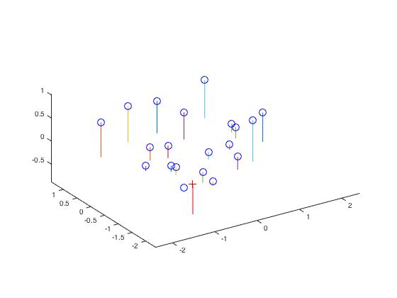
The matrix takes every 3D world point and project it to the 2D homogeneous coordinate on an image before it gets converted into the inhomogeneous coordinate. The M matrix was solved by arranging the problem into a homogeneous linear system and solving the system by linear least square regression. It should be noted that singular value decomposition was used to fix a scale for the M matrix. The residual between the 2D points and the projection of 3D points (through M matrix) is 0.0445. Once the M matrix was obtained, we determined the camera center, C, by the following:
| M = (Q | m4) |
| C = -Q-1 m4 |
| -1.5127 |
| -2.3517 |
| 0.2826 |
The plot below shows the position of the camera relative to various points.
|
Example of code for computer_camera_center.m
%example code
for i=1:size(Points_3D,1)
    X(i) = Points_3D(i,1);
    Y(i) = Points_3D(i,2);
    Z(i) = Points_3D(i,3);
    u(i) = Points_2D(i,1);
    v(i) = Points_2D(i,2);
end
%%
j =1;
for i = 1:1:length(X)
P(j) = X(i);
P(j+1) = Y(i);
P(j+2) = Z(i);
P(j+3) = 1;
P(j+4:j+7) = 0;
P(j+8) = -u(i)*X(i);
P(j+9) = -u(i)*Y(i);
P(j+10) = -u(i)*Z(i);
P(j+11) = -u(i);
P(j+12:j+15) = 0;
P(j+16) = X(i);
P(j+17) = Y(i);
P(j+18) = Z(i);
P(j+19) = 1;
P(j+20) = -v(i)*X(i);
P(j+21) = -v(i)*Y(i);
P(j+22) = -v(i)*Z(i);
P(j+23) = -v(i);
j=j+24;
end

A = im2col(P,[1 12],'distinct')';
[U, S, V] = svd(A);
M = V(:,end);
M = reshape(M,[],3)';
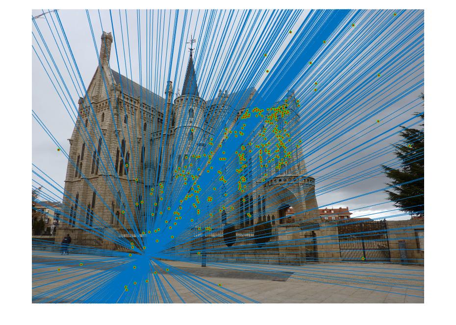
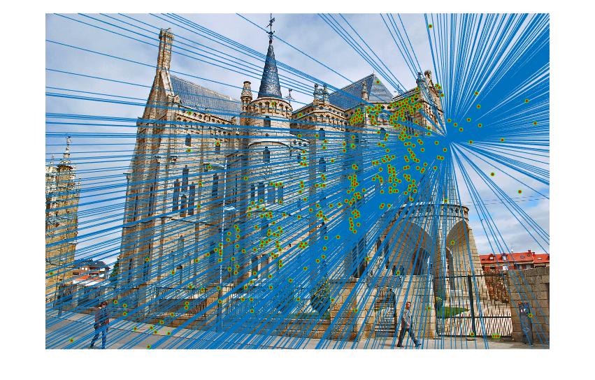
Part 2
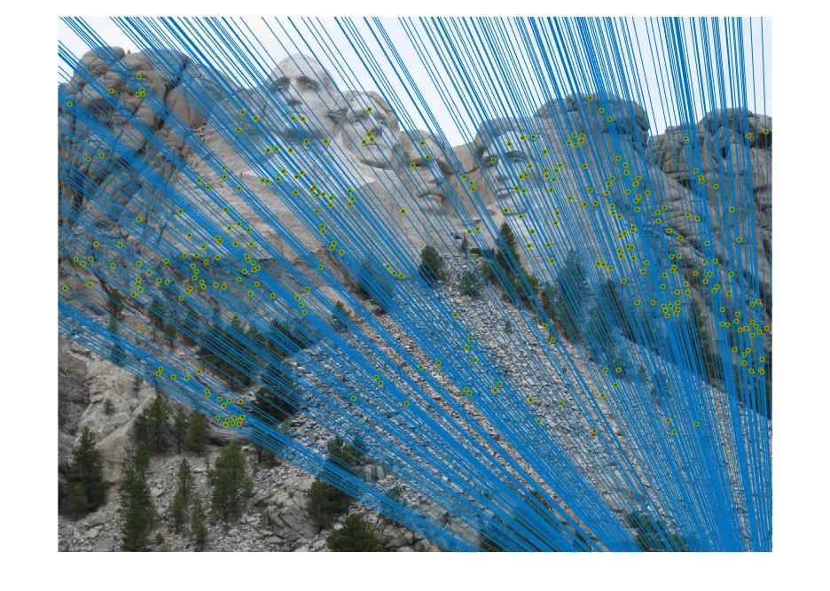
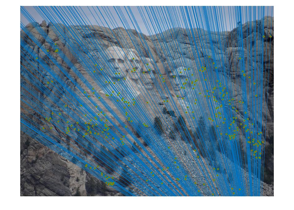
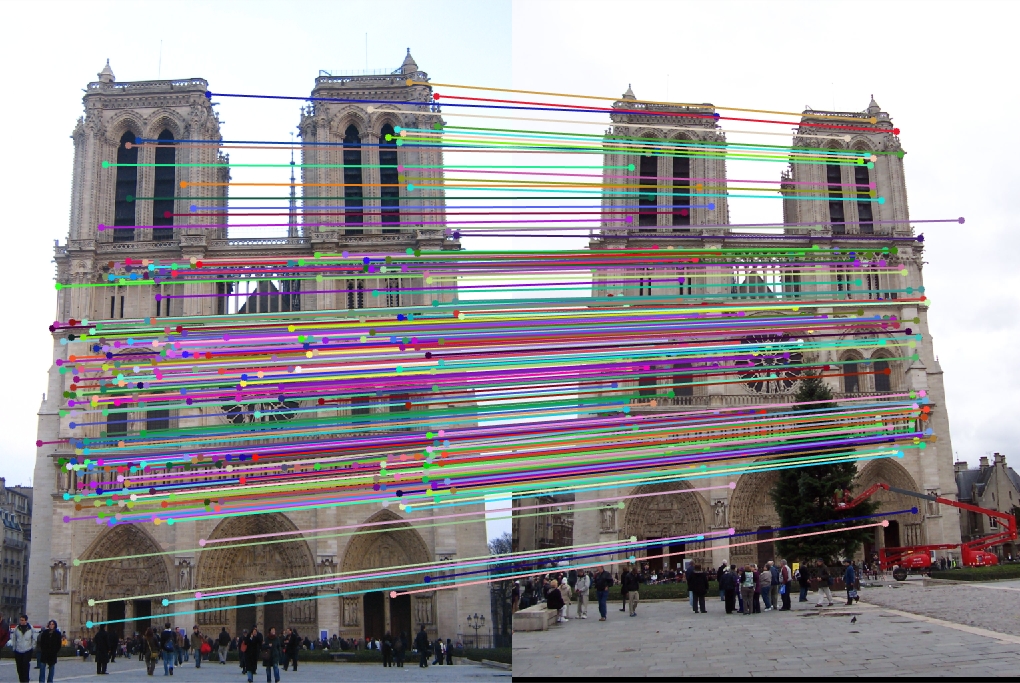
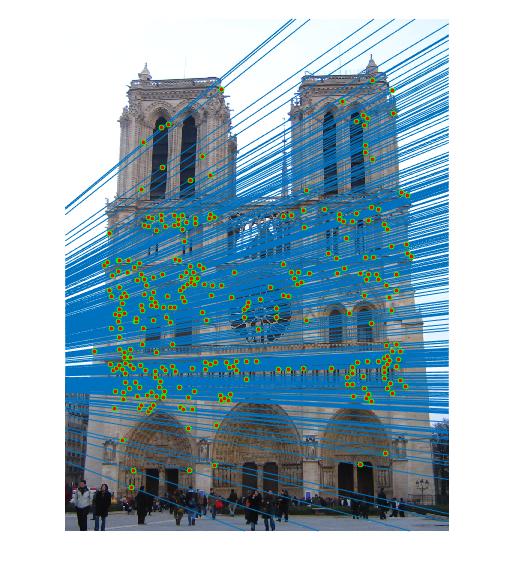
The objective of this part of the project is to perform mapping of points from one image to another image through a fundamental matrix. The fundamental matrix is a 3x3 matrix that directly relates the 2D coordinates from the two images. The linear regression equation systems can be formed from this relationship. The same method of singular value decomposition, used in Part 1, was used to fix the scale for the regression matrix. Besides that, since the fundamental matrix is a rank 2 matrix (determinant of the fundamental matrix is zero), we reduced its rank by setting the smallest eigenvalue in the matrix to zero. This was done by implementing singular value decomposition on the fundamental matrix that was solved in the previous step. The fundamental matrix was then used to plot the epipolar lines between the two images.
The fundamental matrix without coordinate normalization on the base image pair is
| -5.3626e-7 | 7.9036e-6 | -0.0019 |
| 8.8354e-6 | 1.2132e-6 | 0.0172 |
| -9.0738e-4 | -0.0264 | 0.9995 |
The fundamental matrix with coordinate normalization, which will be further explained in the extra credit section below, on the base image pair is:
| -6.2781e-6 | 8.3395e-5 | -0.0210 |
| 5.3851e-5 | -1.5449e-5 | 0.1659 |
| 6.9831e-5 | -0.2259 | 4.7489 |
Example of code for estimate_fundamental_matrix.m
Pa_updated = Points_a;
Pb_updated = Points_b;
for i=1:size(Pa_updated,1)
    u1(i) = Pa_updated(i,1);
    v1(i) = Pa_updated(i,2);
    u2(i) = Pb_updated(i,1);
    v2(i) = Pb_updated(i,2);
end
%%
j = 1;
for i = 1:1:length(u1)
P(j) = u1(i)*u2(i);
P(j+1) = v1(i)*u2(i);
P(j+2) = u2(i);
P(j+3) = u1(i)*v2(i);
P(j+4) = v1(i)*v2(i);
P(j+5) = v2(i);
P(j+6) = u1(i);
P(j+7) = v1(i);
P(j+8) = 1;
j = j+9;
end
A = im2col(P,[1 9],'distinct')';
[U, S, V] = svd(A);
f = V(:,end);
F = reshape(f,[3 3])';

%%%%%%%%%%%%%%%%
[U, S, V] = svd(F);
S(3,3) = 0;
F_matrix = U*S*V';
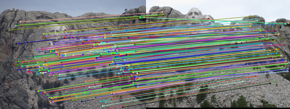
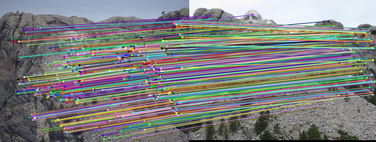
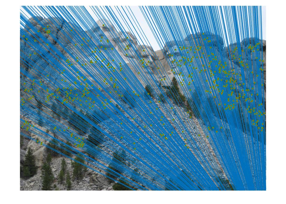
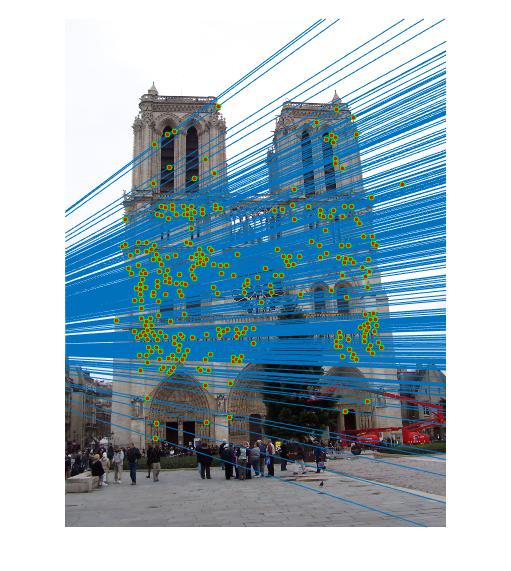
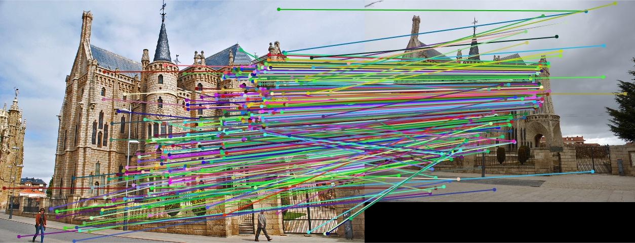
Part 3
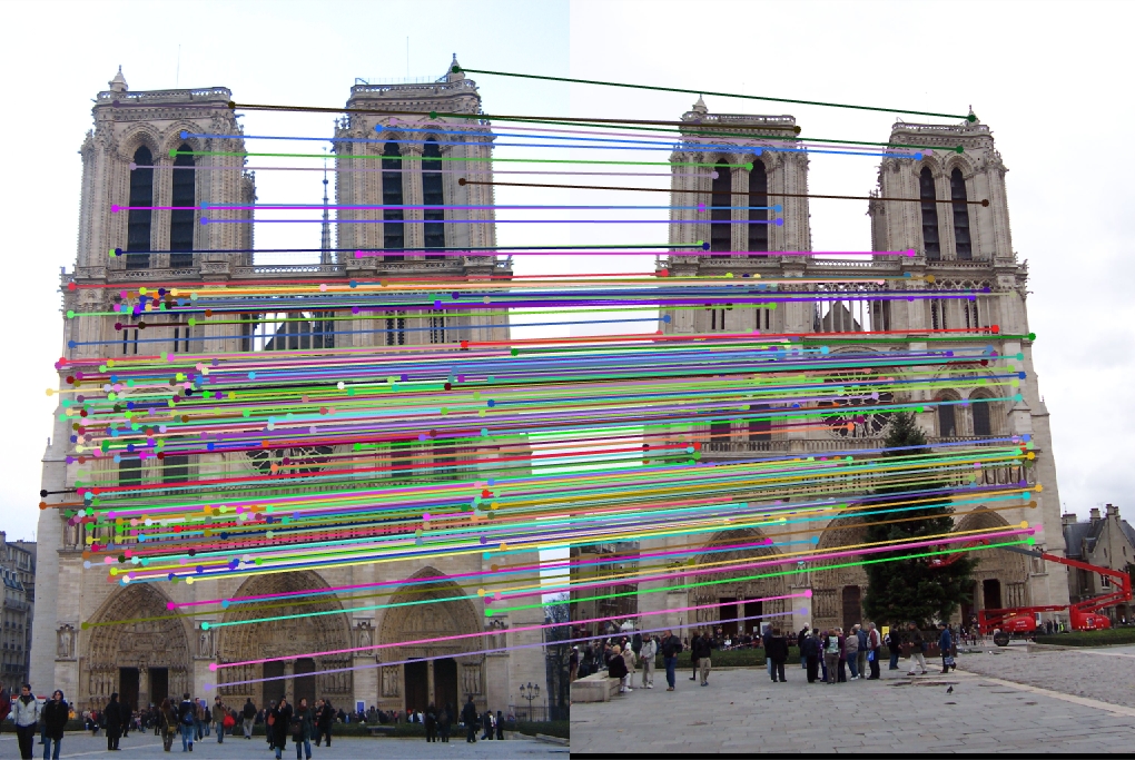
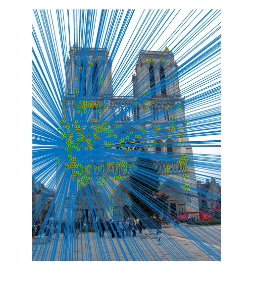
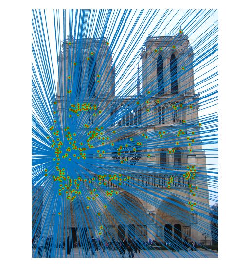
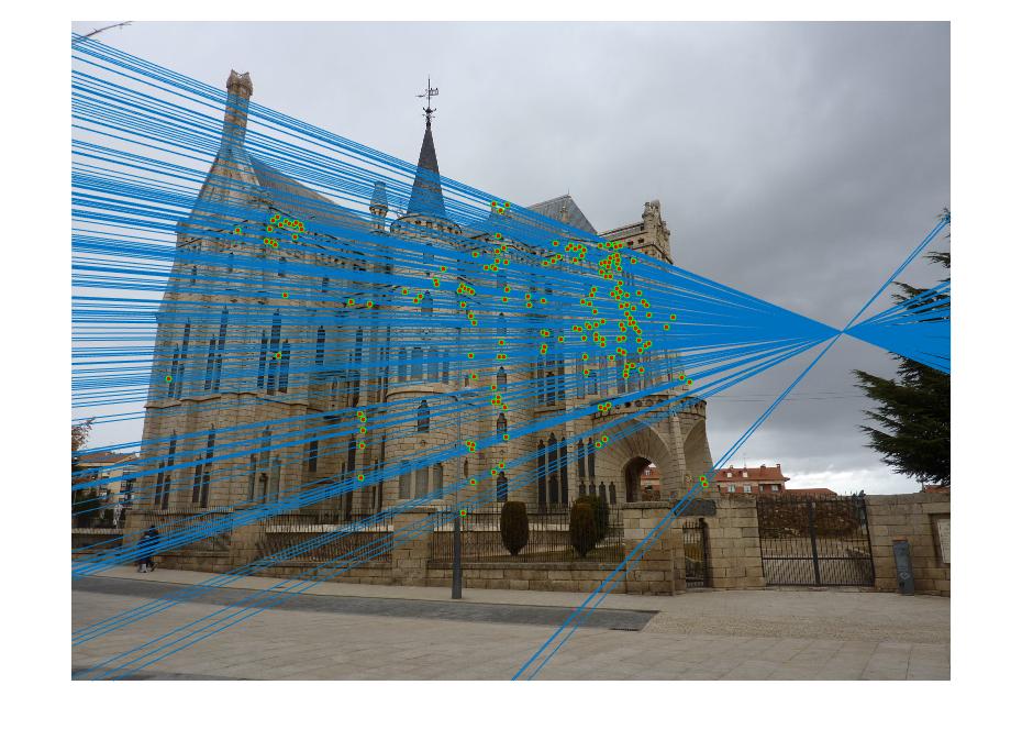
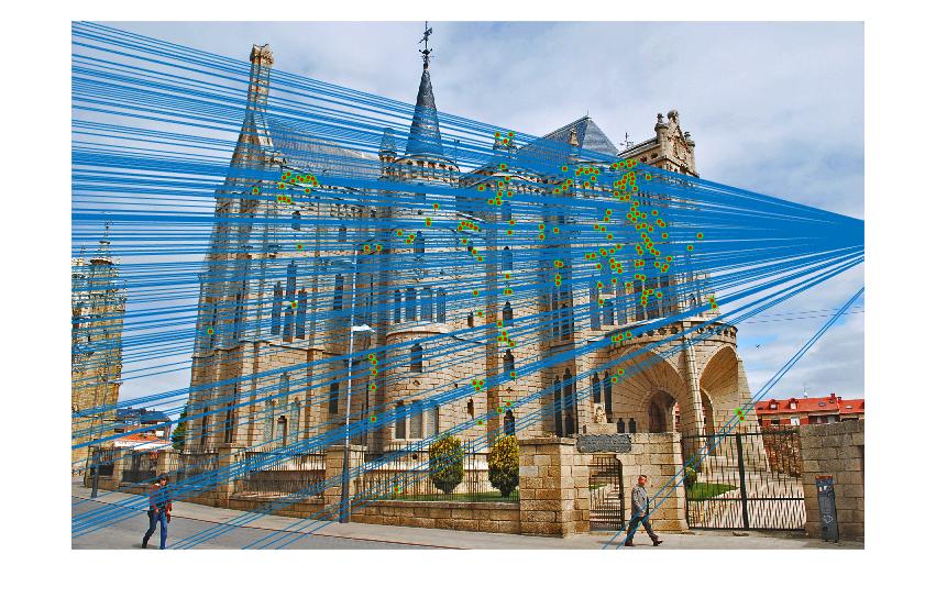
The objective of this part of the project is to perform mapping of points from one image to another image through a fundamental matrix that is optimally determined through RANSAC. We used VLFeat to obtain the SIFT matching features/points from the image pair. The matching point pairs, together with RANSAC algorithm, are used to compute the optimal fundamental matrix. In this process, eight random matching points are used as inputs to the estimate_fundamental_matrix function to compute the fundamental matrix. This is followed by computing the product of the fundamental matrix with the two point correspondences. The point pair are determined as one pair of inliers if the product is smaller than the threshold, which is set to be 0.05. This process goes through 20000 iterations to find the optimal fundamental matrix which leads to the most number of inliers.
Example of code for ransac_fundamental_matrix.m
iteration = 10000;
indexFinal = cell(1,iteration);
numberofsample = 8;
for k = 1:iteration;
n = randsample(size(matches_a,1),numberofsample);
point_a = matches_a(n,:);
point_b = matches_b(n,:);
[F_matrix] = estimate_fundamental_matrix(point_a, point_b);
thres = 2e-2;
q = 1;
for j = 1:size(matches_a,1)
res = [matches_b(j,:) 1]*F_matrix*[matches_a(j,:) 1]';
if abs(res) < thres
index(q) = j;
q = q+1;
end
end
indexFinal{k} = index';
Fmatrixcollection{k} = F_matrix;
vector(k) = length(index);
index=[];
end
[vector2,order] = sort(vector,'descend');
Largest_indexgroup = indexFinal{order(1)};
Best_Fmatrix = Fmatrixcollection{order(1)};
inliers_a = matches_a(Largest_indexgroup,:);
inliers_b = matches_b(Largest_indexgroup,:);
Extra Credit: Normalizing the coordinates of matching features
The estimation of fundamental matrix can be improved by normalizing the coordinates of matching points between the image pair. The normalization process involves finding the mean of the point cloud in each image and subtracting it from each matching point. This shifts the origin to the center of the point cloud. A scaling factor has to be estimated and it was done individually for each image. It is the reciprocal of the average standard deviation of the matching points which have been shifted by subtracting their mean. The scale determined this way was a value of 0.0055. After more tests with the scale, I found that the results were the best when the value of s is 0.5. The normalized fundamental matrix has to be adjusted so that it can operate on the original image coordinates, such that:
| Forig = TbT* Fnorm* Ta |
Example of code for estimate_fundamental_matrix.m with coordinate normalization
%%
% Normalization
% **************************************************
mean_a = mean(Points_a);
c_u1 = mean_a(1);
c_v1 = mean_a(2);
Pa_u = Points_a(:,1)-c_u1;
Pa_v = Points_a(:,2)-c_v1;
Pa = [Pa_u Pa_v];
s1 = 1/mean(std(Pa));
s1 = 0.5;
scaleM1 = [s1 0 0;0 s1 0;0 0 1];
offsetM1 = [1 0 -c_u1;0 1 -c_v1;0 0 1];
Ta = scaleM1*offsetM1;
for i=1:1:size(Points_a,1)
u = Points_a(i,1);
v = Points_a(i,2);
new = scaleM1*offsetM1*[u;v;1];
Pa_updated(i,1) = new(1);
Pa_updated(i,2) = new(2);
end

%%
mean_b = mean(Points_b);
c_u2 = mean_b(1);
c_v2 = mean_b(2);
Pb_u = Points_b(:,1)-c_u2;
Pb_v = Points_b(:,2)-c_v2;
Pb = [Pb_u Pb_v];
s2 = 1/mean(std(Pb));
s2 = 0.5;
scaleM2 = [s2 0 0;0 s2 0;0 0 1];
offsetM2 = [1 0 -c_u2;0 1 -c_v2;0 0 1];
Tb = scaleM2*offsetM2;
for i=1:1:size(Points_b,1)
u = Points_b(i,1);
v = Points_b(i,2);
new = scaleM2*offsetM2*[u;v;1];
Pb_updated(i,1) = new(1);
Pb_updated(i,2) = new(2);
end
% **************************************************
%%

%%
% Pa_updated = Points_a;
% Pb_updated = Points_b;
for i=1:size(Pa_updated,1)
    u1(i) = Pa_updated(i,1);
    v1(i) = Pa_updated(i,2);
    u2(i) = Pb_updated(i,1);
    v2(i) = Pb_updated(i,2);
end
%%
j = 1;
for i = 1:1:length(u1)
P(j) = u1(i)*u2(i);
P(j+1) = v1(i)*u2(i);
P(j+2) = u2(i);
P(j+3) = u1(i)*v2(i);
P(j+4) = v1(i)*v2(i);
P(j+5) = v2(i);
P(j+6) = u1(i);
P(j+7) = v1(i);
P(j+8) = 1;
j = j+9;
end
A = im2col(P,[1 9],'distinct')';
[U, S, V] = svd(A);
f = V(:,end);
F = reshape(f,[3 3])';

%%%%%%%%%%%%%%%%
[U, S, V] = svd(F);
S(3,3) = 0;
F_matrix = U*S*V';

%%
% **************************************************
F_matrix = Tb'*F_matrix*Ta;
% **************************************************
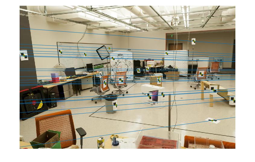
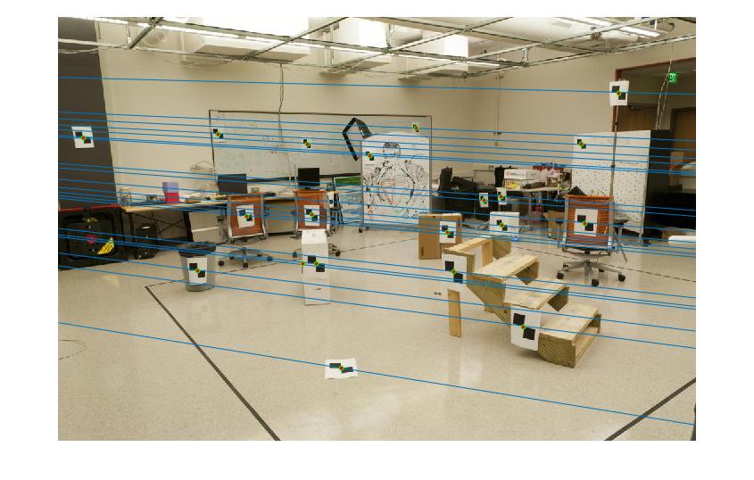
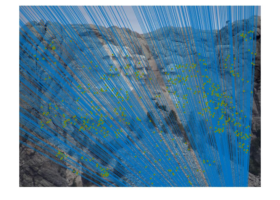
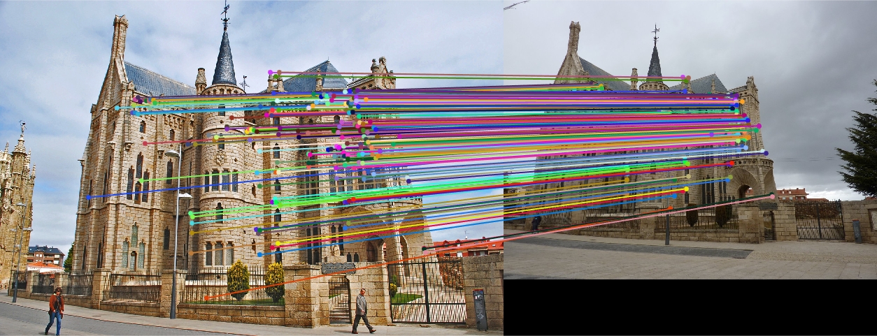
Results in a table (threshold = 0.02; iteration = 100000)
No coordinates normalization

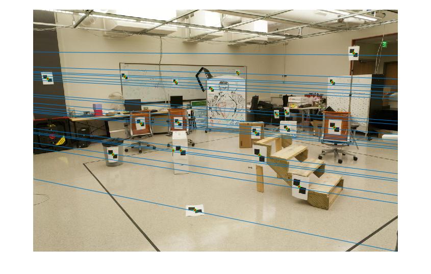 With coordinates normalization
|
No coordinates normalization
 With coordinates normalization
|
No coordinates normalization
 With coordinates normalization
|
No coordinates normalization
 With coordinates normalization
|
It is obvious that coordinate normalization improves the matching of point correspondences between two images through improvement in the fundamental matrix estimation. The effect of coordination normalization is the most significant in the Gaudi example, where the image pair with no coordinate normalization has quite a significant number of incorrect point correspondences while that with coordinate normalization completely eliminates the errors.