Project 3 / Camera Calibration and Fundamental Matrix Estimation with RANSAC
The goal of the project is to map the 3D world coordinates to image coordinates. The next steps are to compute the fundamental martix that relates points in one scene to epipolar lines in another. The camera projection matrix and the fundamental matrix are estimated using point correspondances.
- For the Projection matrix the input is correspoding 3D and 2D points
- For the Fundamental matrix the input is correspoding 2D points across the two images
- The Fundamental matrix was refined using RANSAC to fit the model with the best inliers. This gives us better matching pairs.
Part 1: Computing the Projection matrix and Camera center
- The projection matrix is computed using the formula Ax = 0. These linear regression equations were solved using Singular Value Decomposition.
- The projection matrix after using a scale of -1 is: -0.4583 0.2947 0.0140 -0.0040
0.0509 0.0546 0.5411 0.0524
-0.1090 -0.1783 0.0443 -0.5968
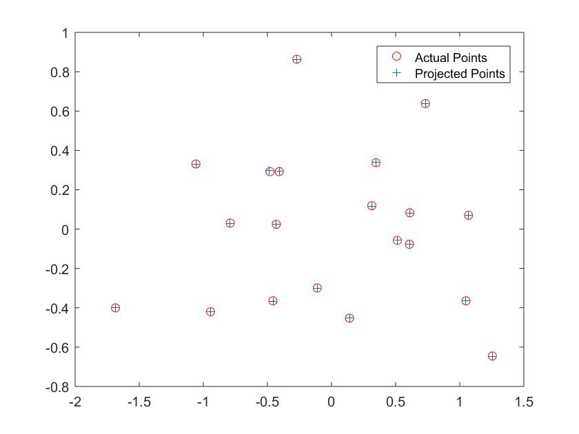
Fig1: Actual and Projected Points
The estimated location of camera is: <-1.5127, -2.3517, 0.2826>
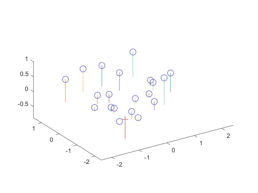
Fig2: Camera Center
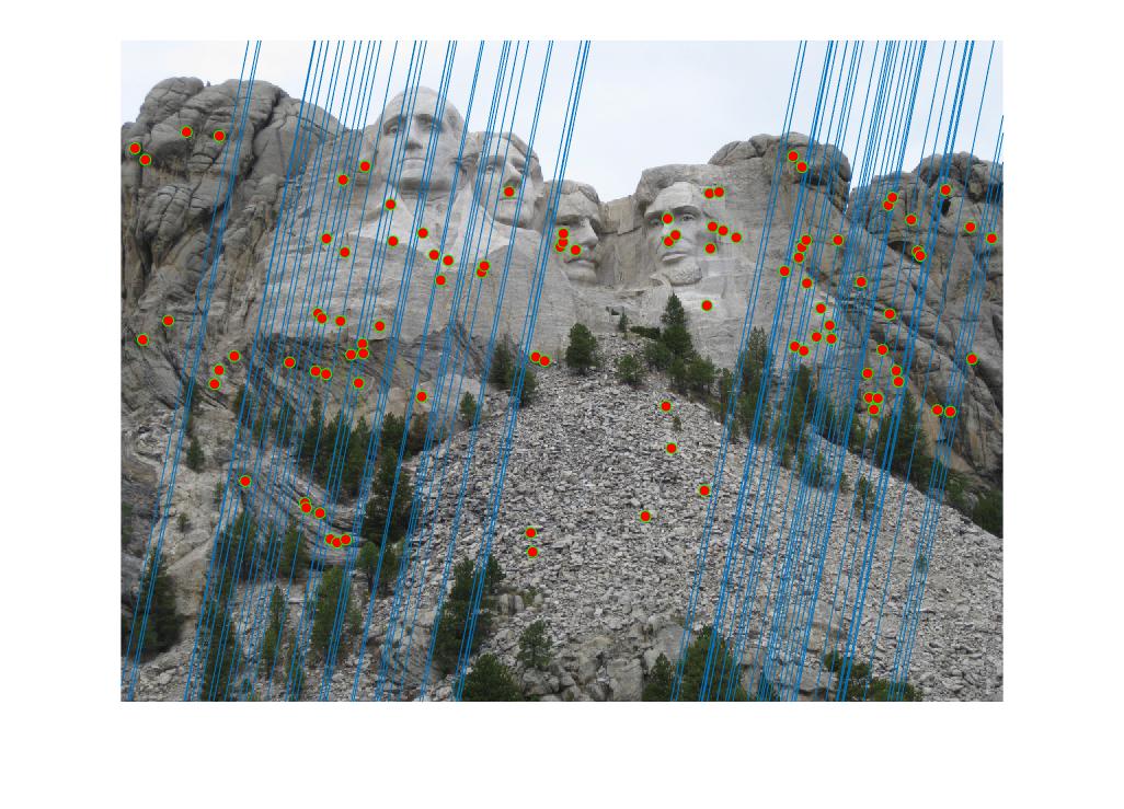
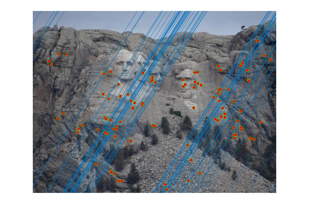
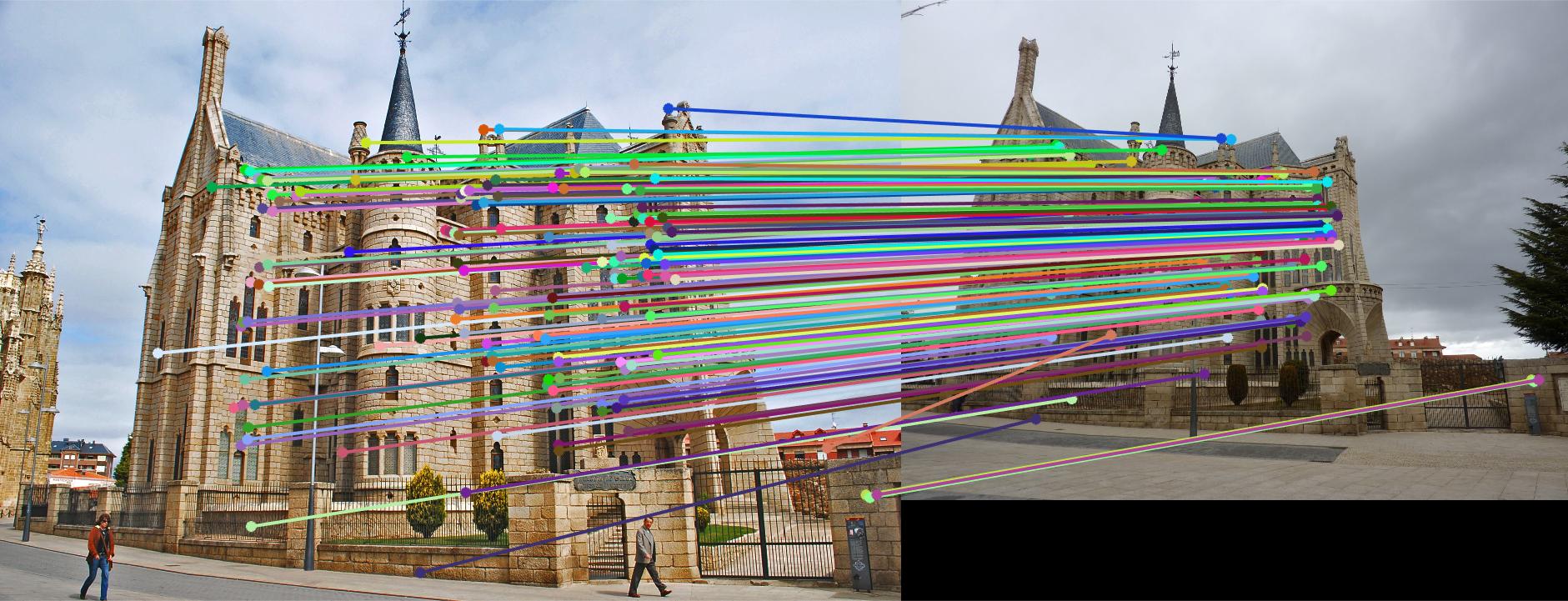
- Use the 2D points from the image pairs and the images themselves. Compute the Fundamental Matrix.Draw the epipolar lines
- The equations correlating the points in the two image planes were setup and SVD was used to solve the linear regression equations.
- I have implemented the normalization of the points before computing the fundamental matrix. This will be discussed in the extra credit section. However, the images below depict the apipolar lines drawn after normalizing the points.
Part 2: Estimating the Fundamental Matrix
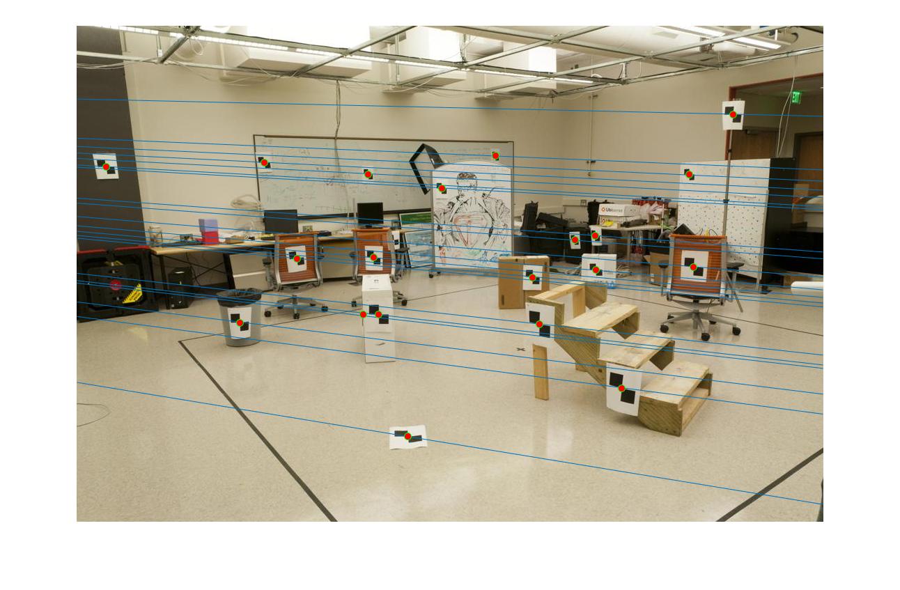
Fig3: Epipolar Lines
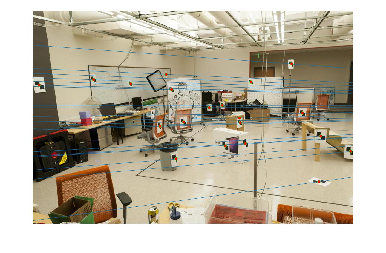
Fig4: Epipolar Lines
Part 2:Estimating the Fundamental Matrix - Normalization (Extra - Graduate Credit)
- The mean values of the points are computed in the u and the vv coordinates
- New points are obtained by subtracting these mean values from the initial points
- Compute the standard deviation along both the coordinates
- Compute the mean of these standard deviation values. Since the initial scale i used was 1, therefore the updated scale i found was 1/mean(standard deviation)
- Compute the transformation matrix and the normalized points. This matrix is then used with the fundamental matrix.
%Finding the mean of the points
mean_u = mean(points_norm(1,finite_indices));
mean_v = mean(points_norm(2,finite_indices));
%Offset by the mean
new_u(1,finite_indices) = points_norm(1,finite_indices)-mean_u; % Shift origin to centroid.
new_v(2,finite_indices) = points_norm(2,finite_indices)-mean_v;
%Find the standard deviation of the points
dist1 = std(new_u,0,2);
dist2 = std(new_v,0,2);
%the distance std matrix
distance = [dist1;dist2];
%Computing scale
std_dist = mean(std(distance));
%The initial scale assumed is 1
scale = 1/std_dist;
%Computing the Transformation matrix and the normalized points
T_matrix = [scale   0   -scale*mean_u;0     scale -scale*mean_v;0       0      1];
normalized_points = T_matrix*points_norm;
Part 2:Estimating the Fundamental Matrix - Normalization (Extra - Graduate Credit)
- The mean values of the points are computed in the u and the vv coordinates
- New points are obtained by subtracting these mean values from the initial points
- Compute the standard deviation along both the coordinates
- Compute the mean of these standard deviation values. Since the initial scale i used was 1, therefore the updated scale i found was 1/mean(standard deviation)
- Compute the transformation matrix and the normalized points. This matrix is then used with the fundamental matrix.
- These normalized points were used in the RANSAC section and produced better results than when the points were not normalized
Part 3:Using RANSAC to estimate the best fundamental matrix
- Randomly sample 8 points from the total number of points
- Compute the fundamental matrix for these points. These points will be normalized while this computation.
- Use the Sampson distance function to obtain the distance.This has been referenced from: https://www.cvg.ethz.ch/teaching/2010fall/compvis/assignments/Exercise4.pdf
- Obtain the best inliers.
- Compute the fundamental matrix for these inliers.
- The best matches correspond to these inliers and the number of inliers depends on the threshold value set.
Results
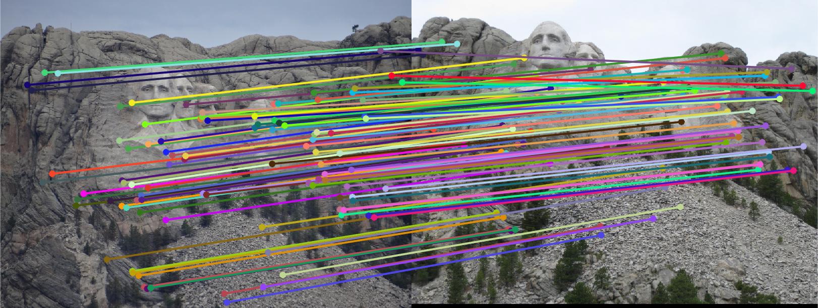
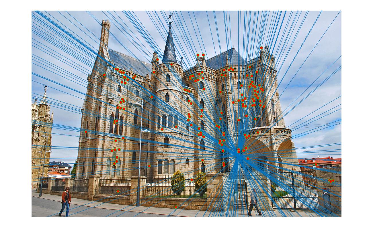
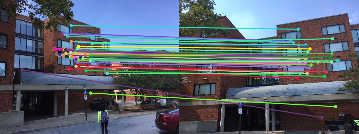
Threshold value: 0.005 - Rushmore
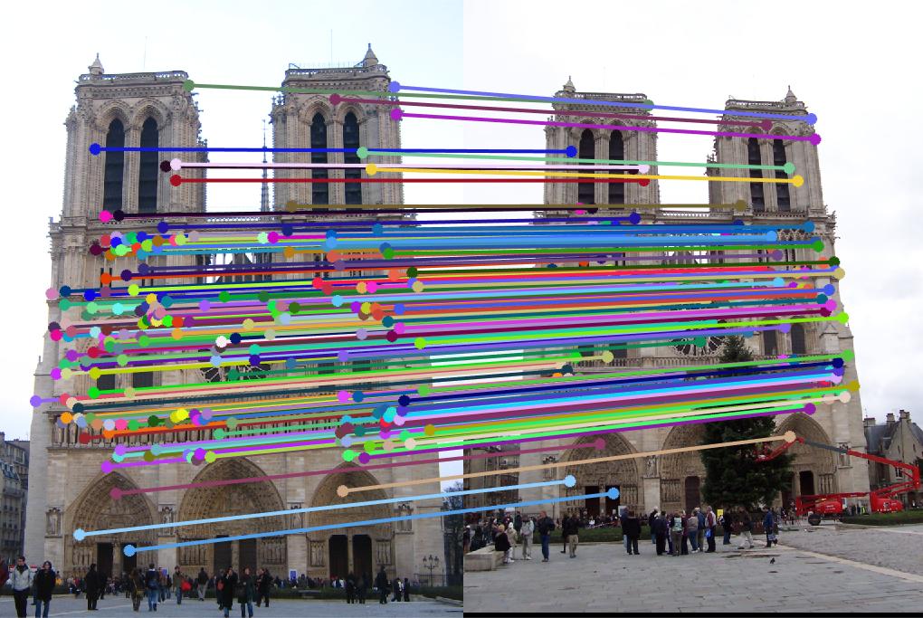
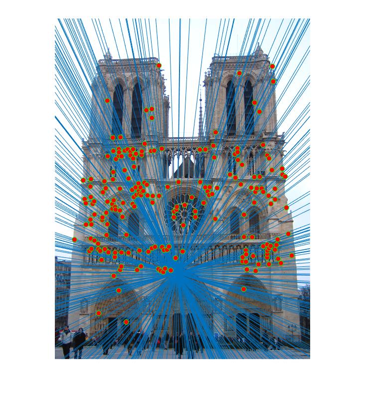
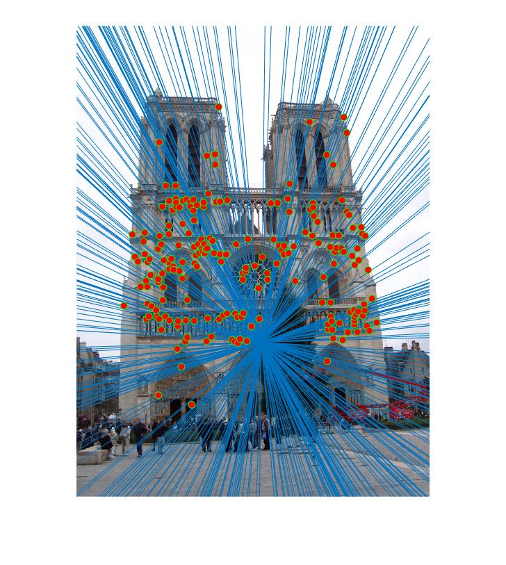
Threshold value: 0.05 - Notre Dam
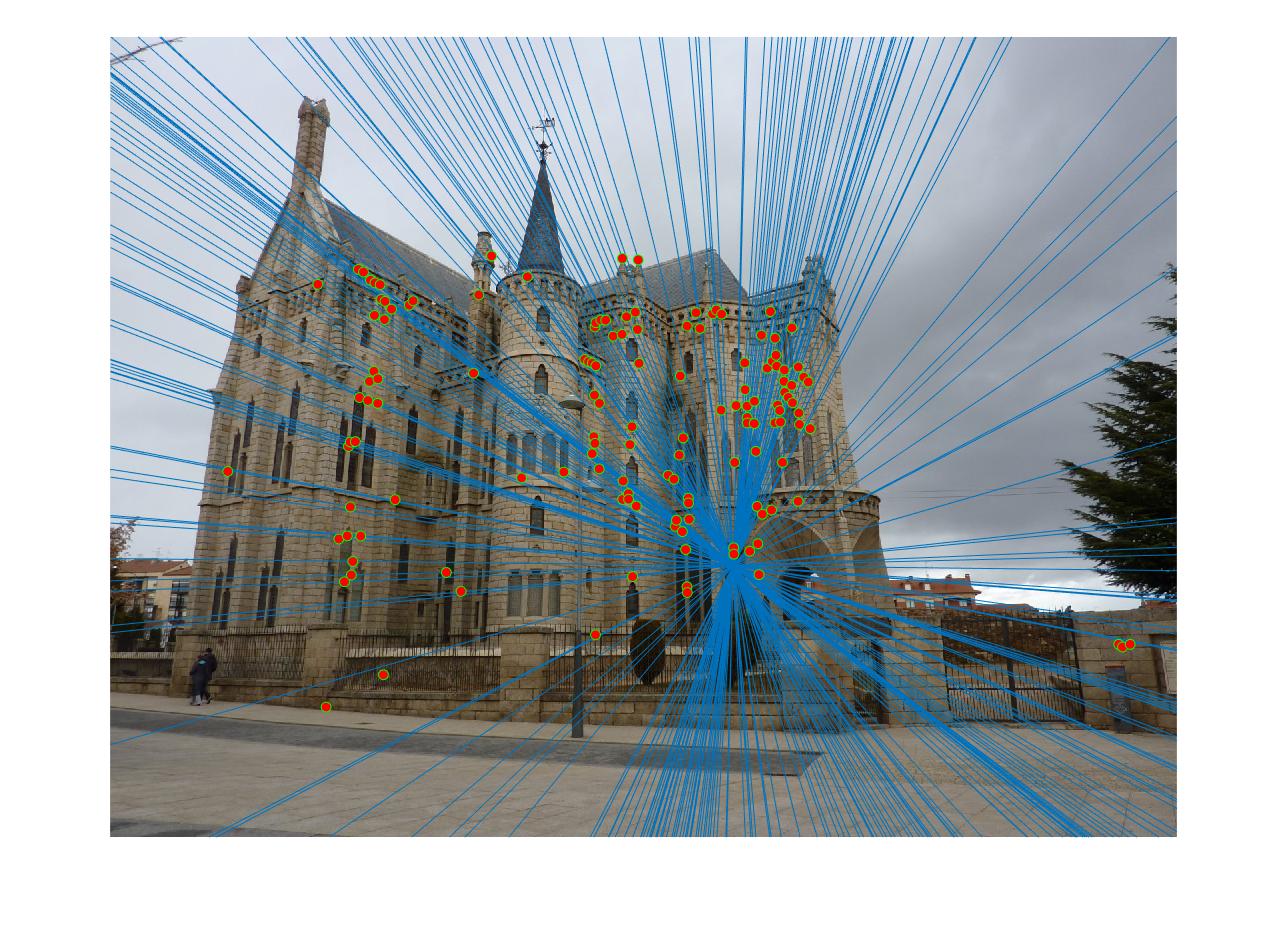
Threshold value: 0.005 - Gaudi
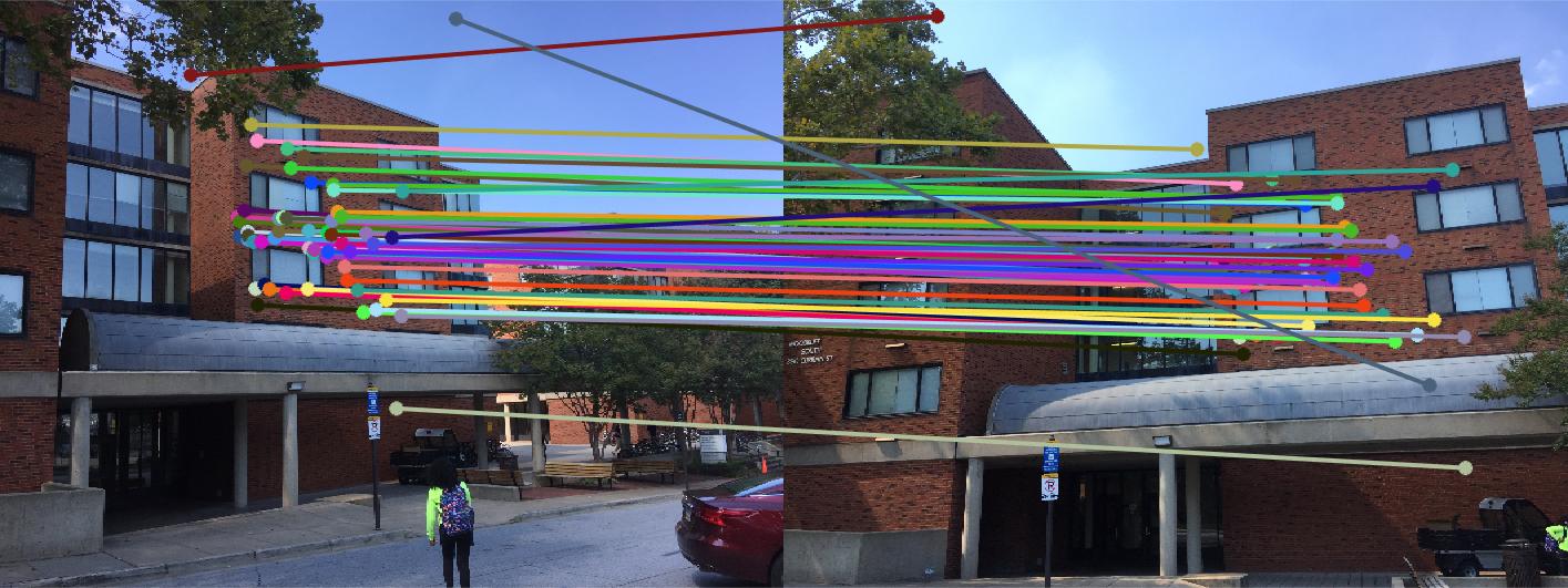
Threshold value: 0.05 - Dorm
|
|
|
|
There are a couple of matches that are not correct as observed from the Results section. However, most of the matches are right due to the fact that they represent the inliers. This is a drastic improvement over computing matches using the interest points and SIFT features concept.
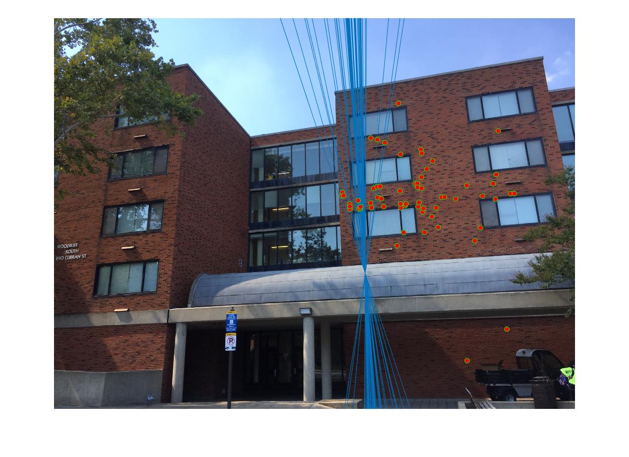
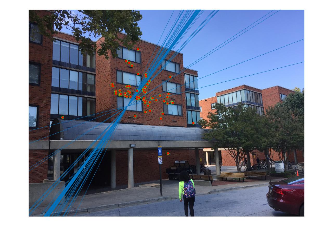
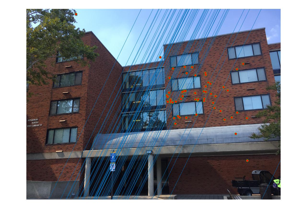
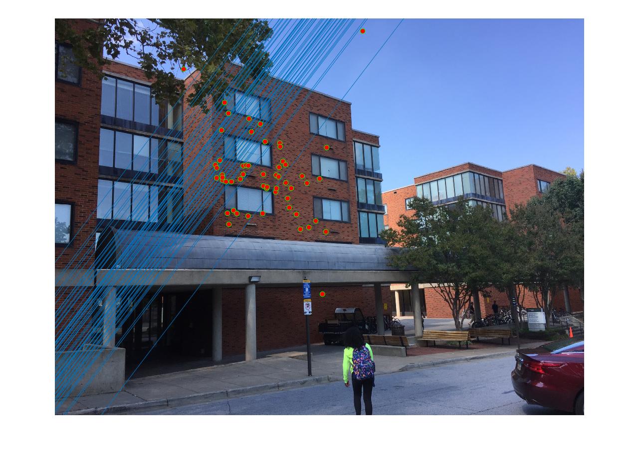
Results - Before and After normalization (Extra Credit)
Observing the difference before and after normalizing the points
|
|
|
The threshold value used for both cases is 0.05. Clearly before normalization, there are many matches that are off by a small distance/value. There are a couple that are way off. But after implementing the normalization portion the matches are configured from the exact spots rather than being around the same "locality". Hence, normalizing points gives a better representation of the matches.
Note: When the code is run with the given threshold values, it may sometimes crash because it may not be able to find the required inliers for those sample points. Although this happens rarely, running the code once more should get it working.The threshold values I have mentioned are strict. Relaxing these values may also help, especially for the Dorm image. Results for this image can be obtained between threshold values of 0.05 to 0.5