Project 3 / Camera Calibration and Fundamental Matrix Estimation with RANSAC
Part 1
Here, we find how 3D world coordinates map to the 2D image coordinates given some ground truth. The projection matrix M is calculated based on the formula given in the project description. The function calculate_projection_matrix takes in the ground truth in terms of the 3D coordinates and the corresponding 2D coordinates they map to. This leads to a homogeneous set of equations for the 12 unknown quantities, which is solved using SVD. The last column of V in the decompositon (which corresponds to the smallest singular value) is used as the solution to the set of equations. The final projection matrix is then built by rearranging the 12 coefficients appropriately.
The camera centre is then computed by taking the inverse of the first three columns of M and multiplying it with its fourth column. The matrix obtained is:
This is the same as the expected output scaled by -1, which is fine because the final output is in terms of homogeneous coordinates, so the actual coordiantes do not change with scale (kx/k is the same as x/1). The camera center is found to be at <-1.5127, -2.3517, 0.2826>, which matches the expected output within floating point error.
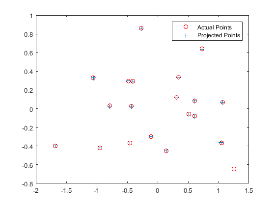
The projections of the 3D points using this obtained matrix are then plotted against the actual positions in the ground truth, as shown below:
Part 2
Here, the fundamental matrix relating two image pairs is found by setting up and solving a system of equations on the lines of what was done in Part 1, except that this matrix relates two sets of 2D points. However, if the 2D coordinates are used as they are, the system has some terms of the form uu' and come terms are simply 1, which leads to a large disparity in numbers since u can be of the order of 103. Hence, normalisation is done in order to bridge this gap. The code for normalisation is shown below:
%%Normalisation
%Mean shifting
Points_a = Points_a - repmat(mean(Points_a),size(Points_a,1),1);

%Estimate the scale
sa = std(Points_a);
Sa = [1/sa(1), 0, 0; 0, 1/sa(2), 0; 0 0 1];

%Actual normalisation
for i=1:size(Points_a)
    scale_a = Sa*[Points_a(i,:) 1]';
    Points_a(i,:) = scale_a(1:2)';
end
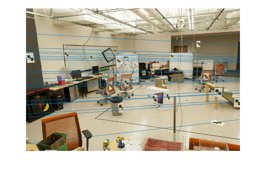
The coordinates are made zero-mean and then their scale is roughly set to 1 by dividing each coordinate by the standard deviation separately along the x and y axes. This is done for both pairs of images and these new coordinates are used to estimate the fundamental matrix. This obtained fundamental matrix is also rescaled appropriately. The matrix obtained after normalisation, and the pairs of epipolar lines before and after normalisation -- which are more accurate -- are shown below:
| Before Normalisation |

|
| After Normalisation |
|
Part 3
Here, I use RANSAC to estimate a fundamental matrix for a pair of images of the same object. The function ransac_fundamental_matrix takes likely pairs of matches between the two images, which very likely have outliers, and uses RANSAC to estimate a fundamental matrix. The inliers with respect to this matrix are separately stored and returned by the visualisation function provided with the starter code.
In the RANSAC algorithm, 8 point pairs are randomly sampled from the matches obtained and the fundamental matrix is estimated like in Part 2. Post-multiplying with Points_a(i,:) will give an epipolar line on Image_b, on which Points_b(i,:) should ideally lie. The distance of the line from this point will give a measure of the `error'. The same can be done for Points_a(i,:) in Image_1 and the two errors can be added (code shown below). All points whose error lies within a threshold are chosen as inliers and the first 30 inliers are returned as matches. The algorithm runs either till a certain number of inliers are found or a specified maximum number of iterations is reached.
%%RANSAC Error Calculation
    for i=1:size(matches_a,1)
        %Find the line and calculate the distance of the corresponding point from it.
        a(:,1)=Current_Fmatrix*[matches_a(i,:), 1]';
        b(:,1)=Current_Fmatrix'*[matches_b(i,:), 1]';
        error1 = abs([matches_b(i,:), 1]*a)/sqrt(a(1,1)^2+a(2,1)^2);
        error2 = abs([matches_a(i,:), 1]*b)/sqrt(b(1,1)^2+b(2,1)^2);
        if error1 + error2 < 2*delta
            num_inliers=num_inliers+1;
            inlier_indices(num_inliers) = i;
        end
    end
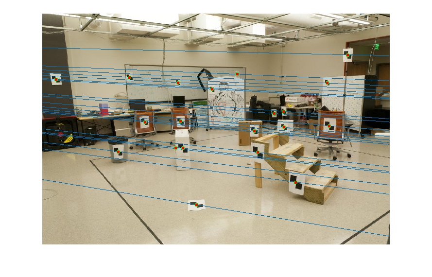
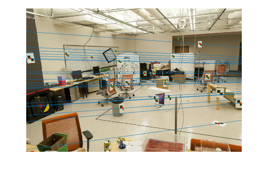
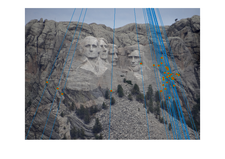
For the Mount Rushmore pair, a sample result and epipolar lines in both image pairs has been shown below.
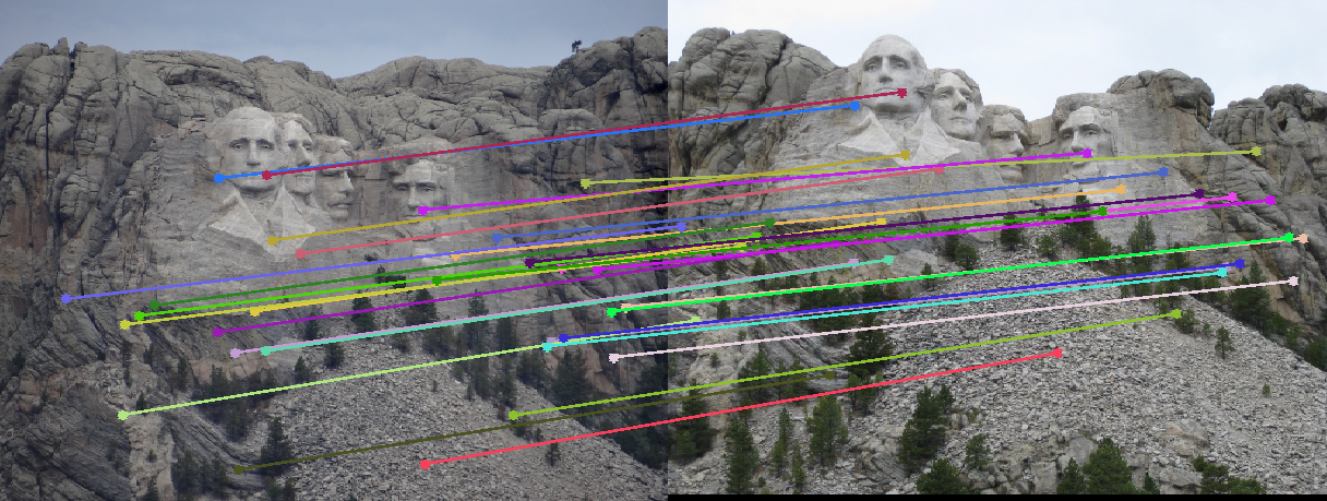

All correspondences seem to match, but even if there was a mismatch, it would have been because the mismatching feature happens to lie on the correct epipolar line at a different place, which would make its error very small and classify it as an inlier. However, since I am checking for errors in both images A and B and adding them, for this to happen both matches will have be wrong and yet lie close to the epipolar lines of each other, which is unlikely. The fundamental matrix obtained was roughly:
Observations (and why I chose certain parameters)
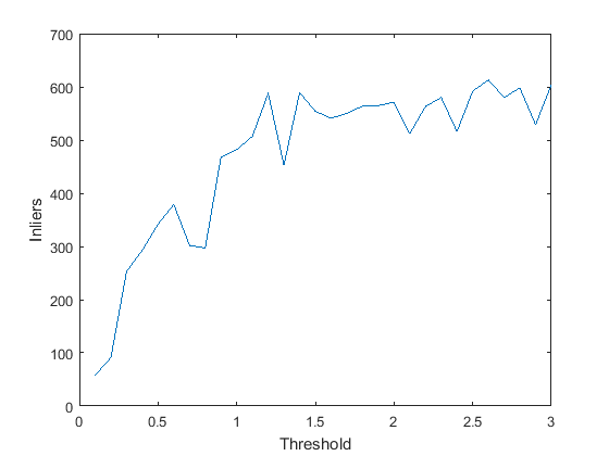
- Error Threshold: At very low values of error threshold (<0.01), the number of inliers obtained is very low. As we increase it, the number of inliers obviously increase, but the rate of increase of inliers will decrease close to a threshold value such that all 'true inliers' have been included and before we start including outliers. A graph showing the number of inliers with increase in the threshold is shown.
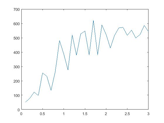
- Effect of Normalisation: The same graph, when plotted without using normalised point coordinates, looks as shown:
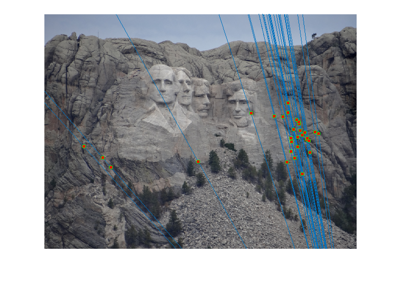
As expected, the epipolar lines with normalisation pass through the inlier points better than the ones without (see extreme right points).Before Normalisation 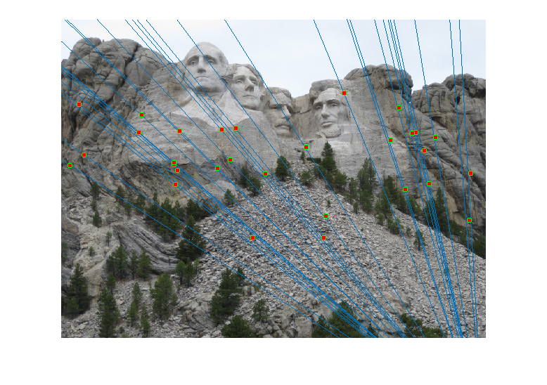
After Normalisation 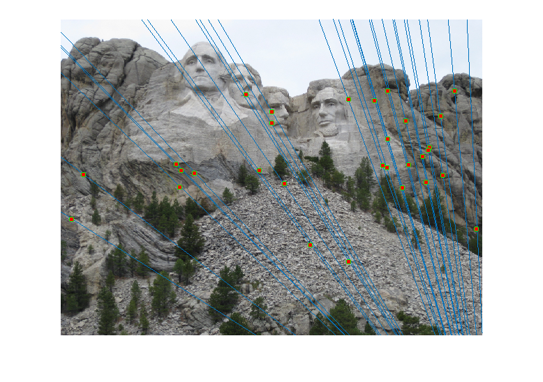
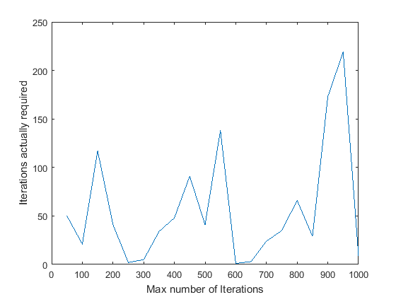
- Max_iterations: I tried varying the max_iterations between 50 and 1000. A graph showing the number of inliers obtained against the number of iterations is shown. Another graph showing the number of iterations the algotithm required before it terminated (inlier_ratio=0.6) is shown.
The algorithm seems to have ended before reaching max_iterations in every case except max_iterations = 50. Also, in every case except that one, the number of inliers obtained is pretty much stabilised close to 550. On an average, it seems to take 100-150 iterations for Mount Rushmore. Based on this, and to be on the safer side, I have set the number of iterations to 400 in the final code.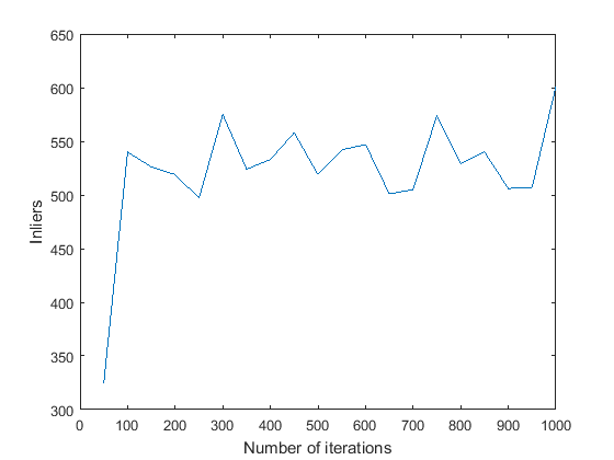
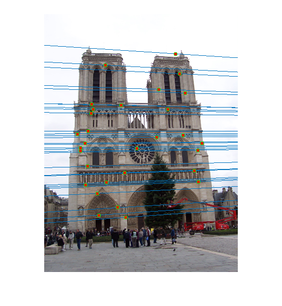
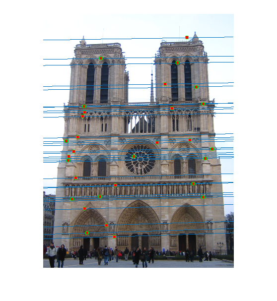
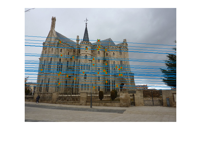
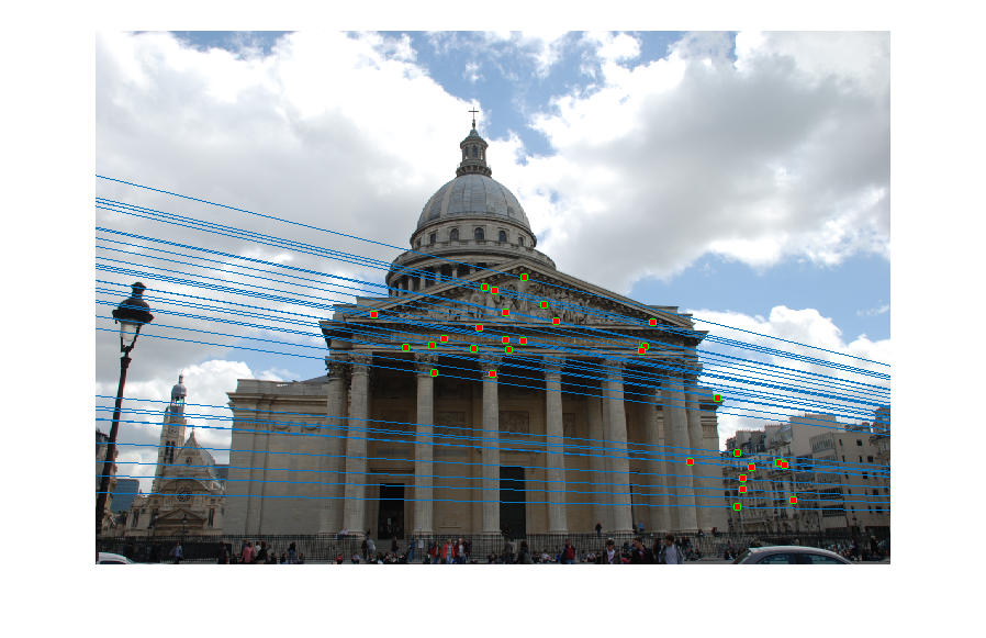
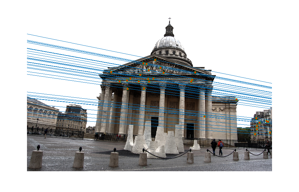
- Different Pairs of Images: The table below shows the results on four different pairs of images.
Image Pair Inliers (Total points) 30 Matches Epipolar lines Notre Dame 530 (851) 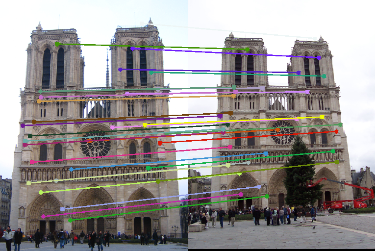
Image 1 Image 2 Gaudi 193 (1062) 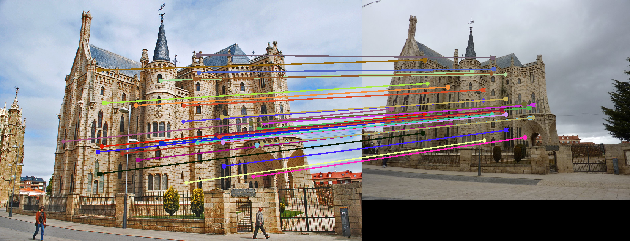
Image 1 Image 2 Pantheon 181 (436) 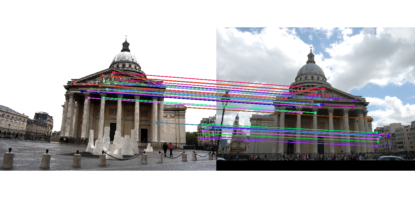
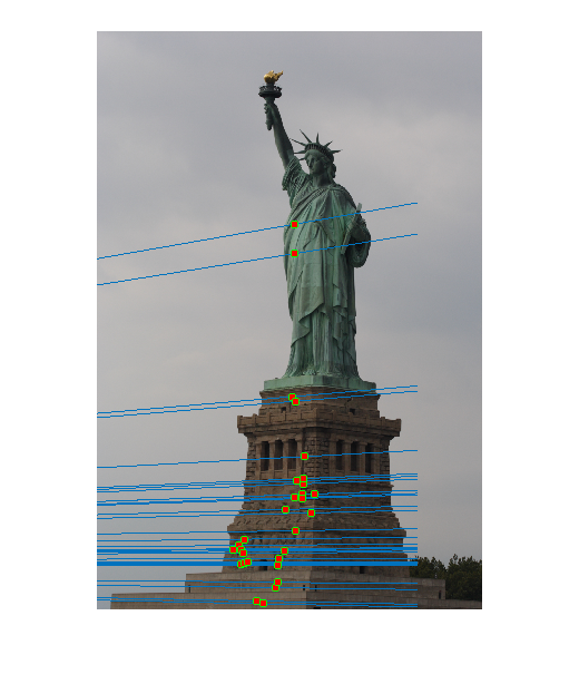
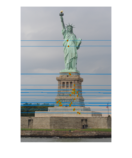
Image 1 Image 2 Statue of Liberty 91 (575) 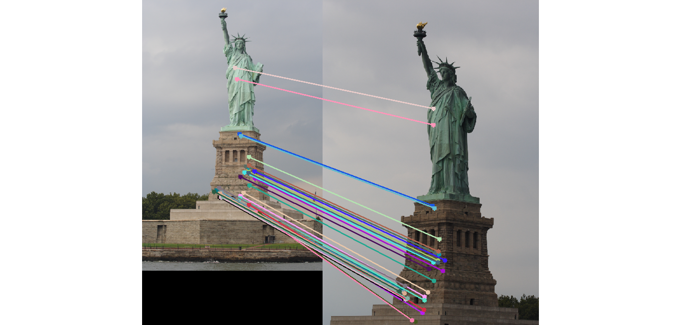
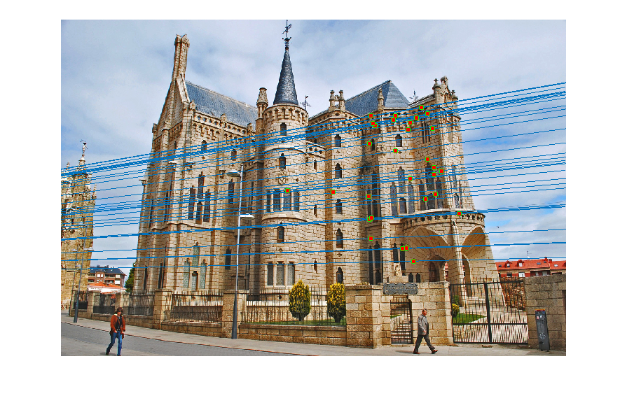
Image 1 Image 2 - Reestimating Fundamental Matrix: Reestimating the fundamental matrix from the obtained 30 inliers seemed to give different epipolar lines occasionally for the Gaudi pair. This may be because the inliers obtained might have had an outlier which was removed when using the 30 random points to reestimate the fundamental matrix. One such case when it happened is shown below:
However, I did not observe this with Mount Rushmore or Notre Dame which probably indicates that those are more accurate estimates of the fundamental matrix.Output of RANSAC 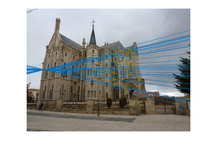
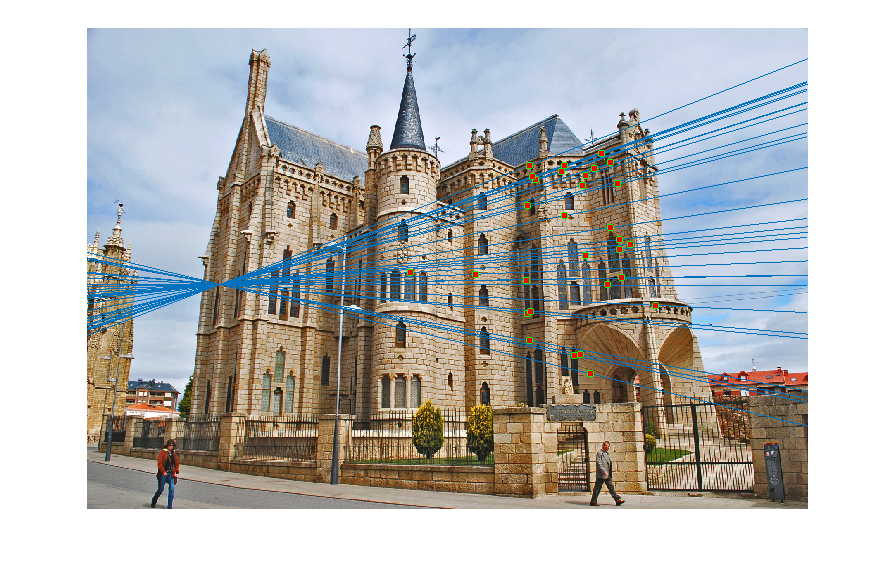
Reestimating with inliers 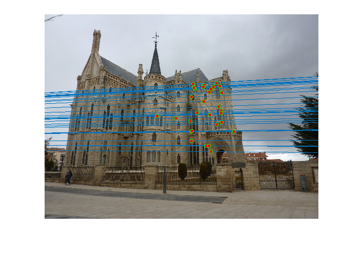
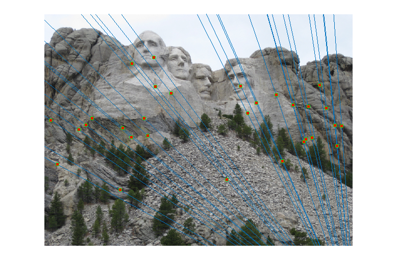
- Choosing more than 8 points: This came as a bit of a surprise. I expected the estimates to get worse if we used more than the minimum (8 points) required for estimating the fundamental matrix, since we now increase the chance of choosing an outlier. However, I got accurate estimates -- with epipolar lines same as the ones shown above -- when I used 12, 16, 24 and even up to 32 points. I did not change any other parameter like the error threshold. Here is an estimate of the epipolar lines calculated for a RANSAC which uses 48 points to calculate the fundamental matrix! It still seems fairly accurate. The number of inliers obtained in this case were 129 (as opposed to 500~600 when I used 8 points).
RANSAC with 48 points 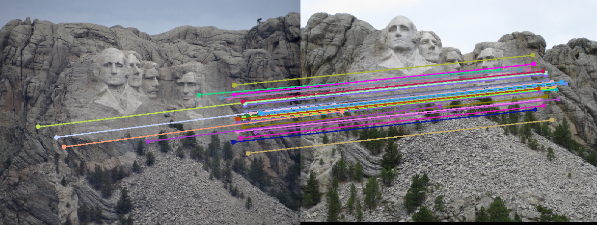
Epipolar Lines for this case 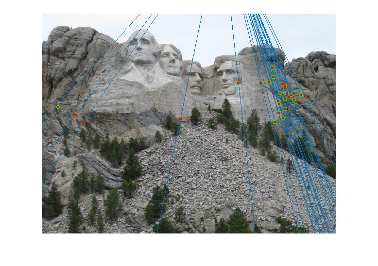
Reestimating F with 30 Random Inliers 
Conclusion
The above report demonstrates an algorithm to estimate the fundamental matrix and with its help obtain accurate matches between pairs of images.