Computer Vision Project

Project 3: Camera Calibration and Fundamental Matrix Estimation with RANSAC

Overview

The goal of this project is to get an introduction to camera and scene geometry. Specifically we will estimate the camera projection matrix, which maps 3D world coordinates to image coordinates, as well as the fundamental matrix, which relates points in one scene to epipolar lines in another. The camera projection matrix and the fundamental matrix can each be estimated using point correspondences. To estimate the projection matrix (camera calibration), the input is corresponding 3d and 2d points. To estimate the fundamental matrix the input is corresponding 2d points across two images. First, we estimate the projection matrix and the fundamental matrix for a scene with ground truth correspondences. Then, we move on to estimating the fundamental matrix using point correspondences from from SIFT.

Part I: Camera Projection Matrix

The goal is to compute the projection matrix that goes from world 3D coordinates to 2D image coordinates. Recall that using homogeneous coordinates the equation for moving from 3D world to 2D camera coordinates is:

$\begin{pmatrix}u \\ v \\ 1\end{pmatrix} \cong \begin{pmatrix}u*s \\ v*s \\ s \end{pmatrix}= \begin{pmatrix}m_{11} & m_{12} & m_{13} & m_{14} \\ m_{21} & m_{22} & m_{23} & m_{24} \\ m_{31} & m_{32} & m_{33} & m_{34} \end{pmatrix} \begin{pmatrix}X \\ Y \\ Z \\ 1 \end{pmatrix}$

Another way of writing this equation is:

$u = \frac{m_{11}X + m_{12}Y + m_{13}Z + m_{14}}{m_{31}X + m_{32}Y + m_{33}Z + m_{34}}$

$\rightarrow (m_{31}X + m_{32}Y + m_{33}Z + m_{34})u = m_{11}X + m_{12}Y + m_{13}Z + m_{14}$

$\rightarrow 0 = m_{11}X + m_{12}Y + m_{13}Z + m_{14} - m_{31}uX - m_{32}uY - m_{33}uZ - m_{34}u$

$v = \frac{m_{21}X + m_{22}Y + m_{23}Z + m_{24}}{m_{31}X + m_{32}Y + m_{33}Z + m_{34}}$

$\rightarrow (m_{31}X + m_{32}Y + m_{33}Z + m_{34})v = m_{21}X + m_{22}Y + m_{23}Z + m_{24}$

$\rightarrow 0 = m_{21}X + m_{22}Y + m_{23}Z + m_{24} - m_{31}vX - m_{32}vY - m_{33}vZ - m_{34}v$

At this point, we are almost able to set up linear regression to find the elements of the matrix M. There's only one problem, the matrix M is only defined up to a scale. So these equations have many different possible solutions, in particular M = all zeros is a solution which is not very helpful in our context. The way around this is to first fix a scale and then do the regression. There are several options for doing this. We can fix the last element ( $m_{34}$ ) to 1 and then find the remaining coefficients, or we can use singular value decomposition to directly solve the constrained optimization problem:

$\begin{align*} &\min\|Ax \| \\ &s.t ~ \| x \| = 1\end{align*}$

Here, we have chosen to directly solve the above constrained optimization problem using singular value decomposition.

The first task was to write the least squares regression to solve for M given the corresponding normalized points. Our code sets up the linear system of equations, solves for the unknown entries of M, and reshapes it into the estimated projection matrix. Once we have an accurate projection matrix M, it is possible to tease it apart into the more familiar and more useful matrix K of intrinsic parameters and matrix [R | T] of extrinsic parameters. Here, we estimate one particular extrinsic parameter: the camera center in world coordinates. Let us define M as being made up of a 3x3 we’ll call Q and a 4th column will call $m_{4}$ :

$M = (Q | m_4 )$

The center of the camera C can be found by:

$C = -Q^{-1} m_4$

The relevant code snippet is shown below:

function M = calculate_projection_matrix( Points_2D, Points_3D )

A = [];
for i = 1:size(Points_2D, 1)
   uv = Points_2D(i, :);
   u = uv(1);
   v = uv(2);
   xyz = Points_3D(i, :);
   
   A = [xyz 1 0 0  0  0 -u.*xyz -u;
         0  0 0 0 xyz 1 -v.*xyz -v;
         A];
end

[~, ~, V] = svd(A);
M = V(:, end);
M = reshape(M, [], 3)';

end

function [ Center ] = compute_camera_center( M )

Q = M(:, 1:3);
m4 = M(:, 4);
Center = -inv(Q) * m4;

end

The output is shown below:

The projection matrix is:
   -0.4583    0.2947    0.0140   -0.0040
    0.0509    0.0546    0.5411    0.0524
   -0.1090   -0.1783    0.0443   -0.5968


The total residual is: 0.0445

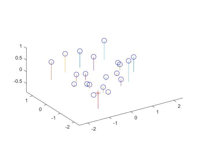
The estimated location of camera is: -1.5127, -2.3517, 0.2826

The reference matrix M and the camera centre are shown below:

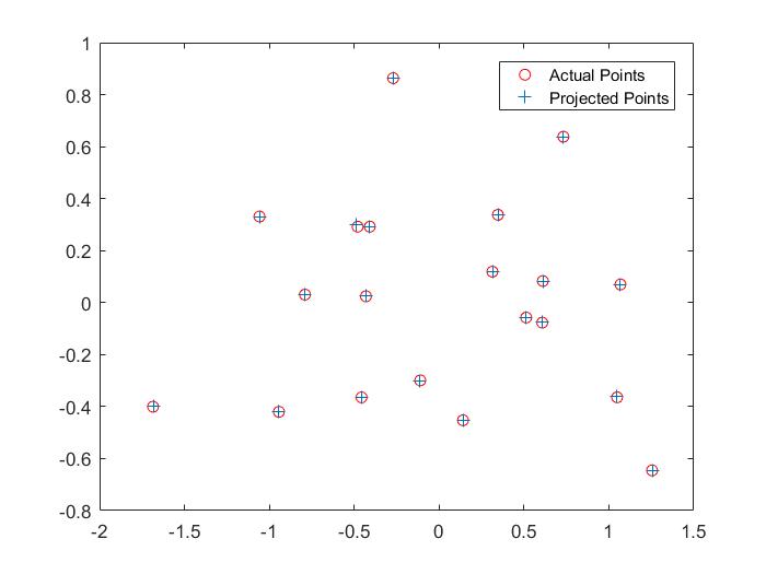
$M_{\text{norm}A} = \begin{pmatrix}-0.4583 & 0.2947 & 0.0139 & -0.0040 \\ 0.0509 & 0.0546 & 0.5410 & 0.0524 \\ -0.1090 & -0.1784 & 0.0443 & -0.5968 \end{pmatrix}$

$C_{\text{norm}A} = < -1.5125, -2.3515, 0.2826 >$

Here are visualizations which show the estimated 3d location of the camera with respect to the normalized 3d point coordinates and a comparison between the projected points and the corresponding actual points.

Part II: Fundamental Matrix Estimation

Now, we estimate the mapping of points in one image to lines in another by means of the fundamental matrix. We will make use of the corresponding point locations listed in pts2d-pic_a.txt and pts2d-pic_b.txt. The definition of the Fundamental Matrix is:

$\begin{pmatrix}u' & v' & 1\end{pmatrix}\begin{pmatrix}f_{11} & f_{12} & f_{13} \\ f_{21} & f_{22} & f_{23} \\ f_{31} & f_{32} & f_{33} \end{pmatrix} \begin{pmatrix}u \\ v \\ 1\end{pmatrix} = 0$

And another way of writing these matrix equations is:

$\begin{pmatrix}u' & v' & 1\end{pmatrix}\begin{pmatrix}f_{11}u + f_{12}v + f_{13} \\ f_{21}u + f_{22}v + f_{23} \\ f_{31}u + f_{32}v + f_{33} \end{pmatrix} = 0$

Which is the same as:

$\begin{pmatrix}f_{11}uu' + f_{12}vu' + f_{13}u' + f_{21}uv' + f_{22}vv' + f_{23}v' + f_{31}u + f_{32}v + f_{33} \end{pmatrix} = 0$

Given corresponding points, we get one equation per point pair. With 8 or more points we can solve this system of equations. As in part I, there is an issue here where the matrix is only defined up to scale and the degenerate zero solution solves these equations. So we need to solve using the same method we used in part I of first fixing the scale and then solving the regression.

The least squares estimate of F is full rank; however, the fundamental matrix is a rank 2 matrix. As such we must reduce its rank. In order to do this, we can decompose F using singular value decomposition into the matrices $U \Sigma V' = F$ . We can then estimate a rank 2 matrix by setting the smallest singular value in $\Sigma$ to zero thus generating $\Sigma_{2}$ . The fundamental matrix is then easily calculated as $F = U \Sigma_{2} V'$ . 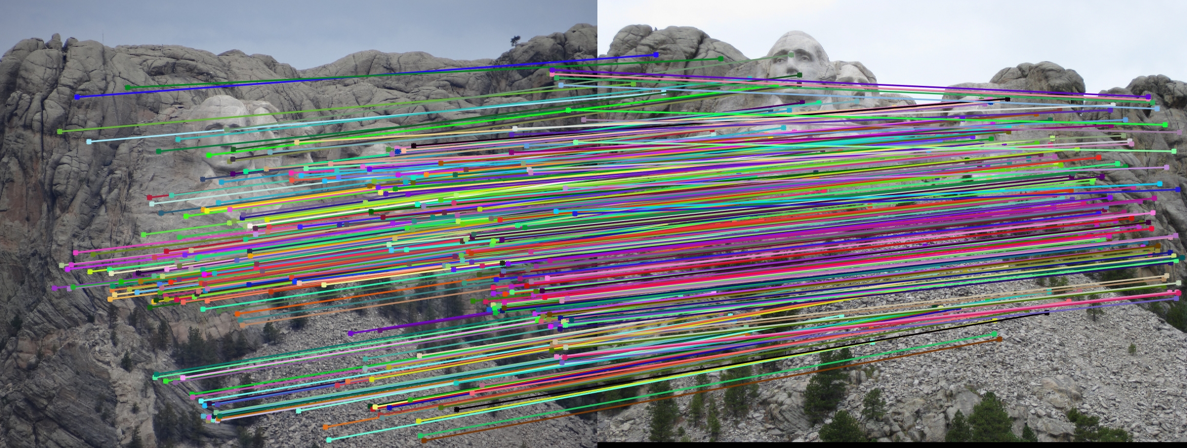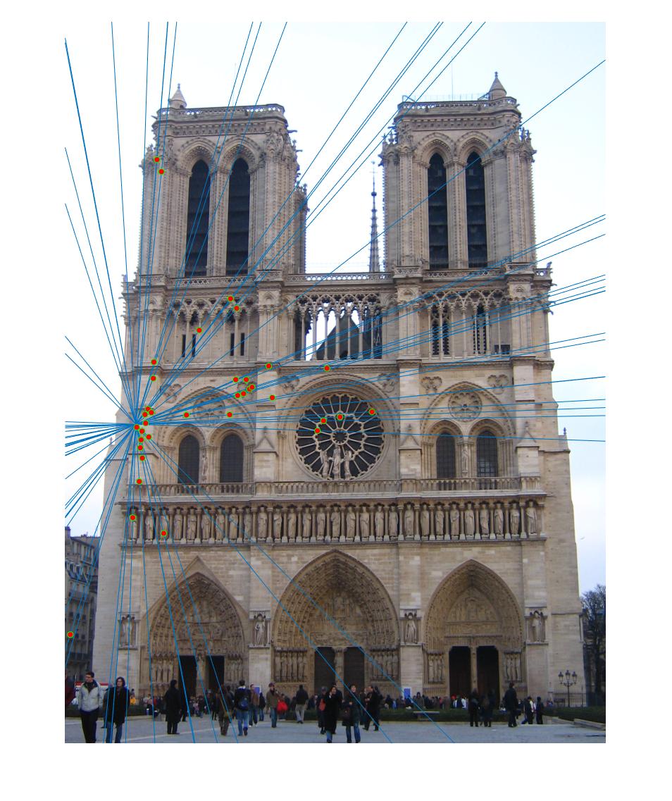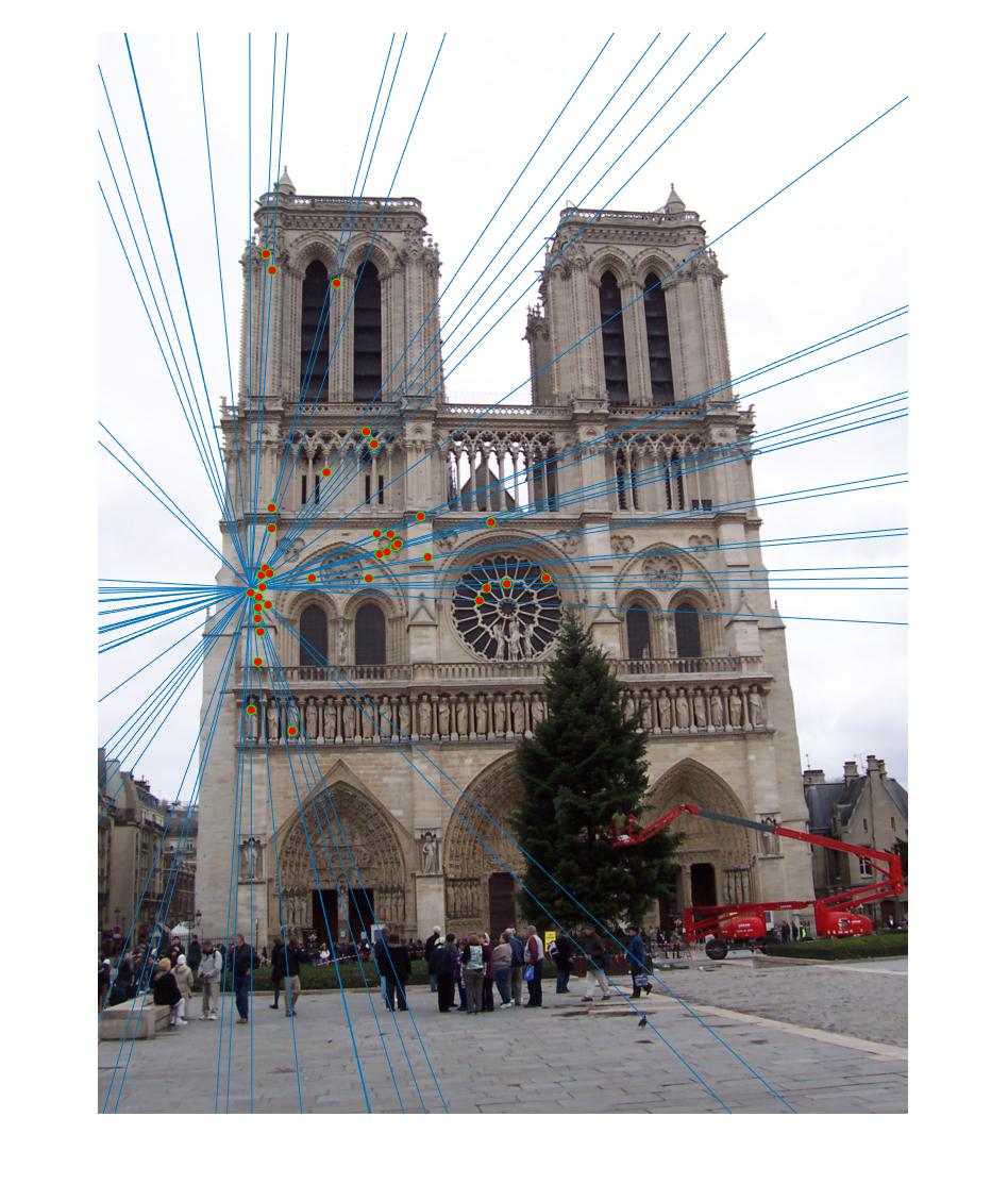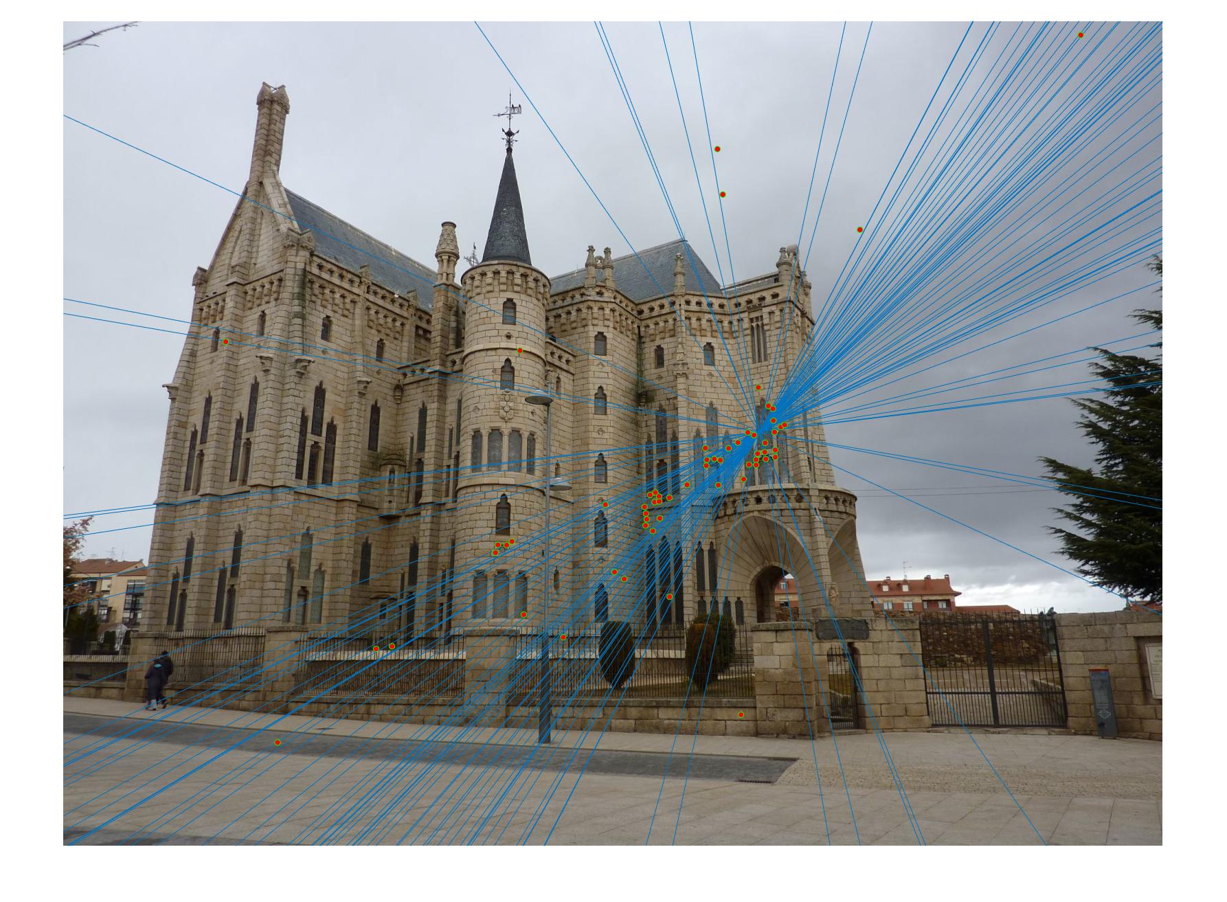We then check the fundamental matrix estimation by plotting epipolar lines.

The relevant code snippet is shown below. Note that we also normalize the fundamental matrix which is discussed in a later section.

function [ F_matrix ] = estimate_fundamental_matrix(Points_a, Points_b)

norm_a = get_normalization_matrix(Points_a);
norm_b = get_normalization_matrix(Points_b);

Points_a = [Points_a ones(size(Points_a, 1), 1)] * norm_a';
Points_b = [Points_b ones(size(Points_b, 1), 1)] * norm_b';

u = Points_b(:, 1);
v = Points_b(:, 2);

A = [repmat(u,1,3) .* Points_a, repmat(v,1,3) .* Points_a, Points_a];

[~, ~, V] = svd(A);
f = V(:, end);
F_matrix = reshape(f, [3 3])';

[U, S, V] = svd(F_matrix);
S(3,3) = 0;
F_matrix = U*S*V';

F_matrix = norm_b' * F_matrix * norm_a;
        
end

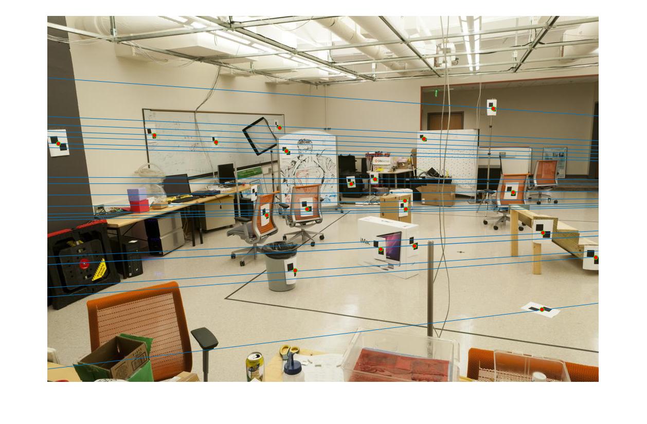
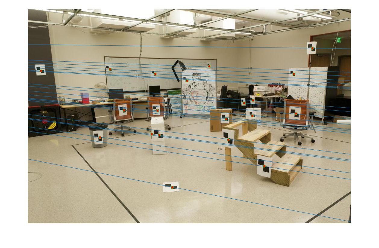
The estimated fundamental matrix for the base pair of images is given below.

F_matrix =

    0.0000   -0.0000    0.0003
   -0.0000   -0.0000   -0.0028
    0.0001    0.0045   -0.1795

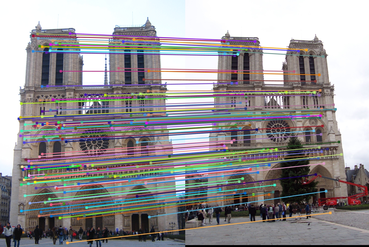
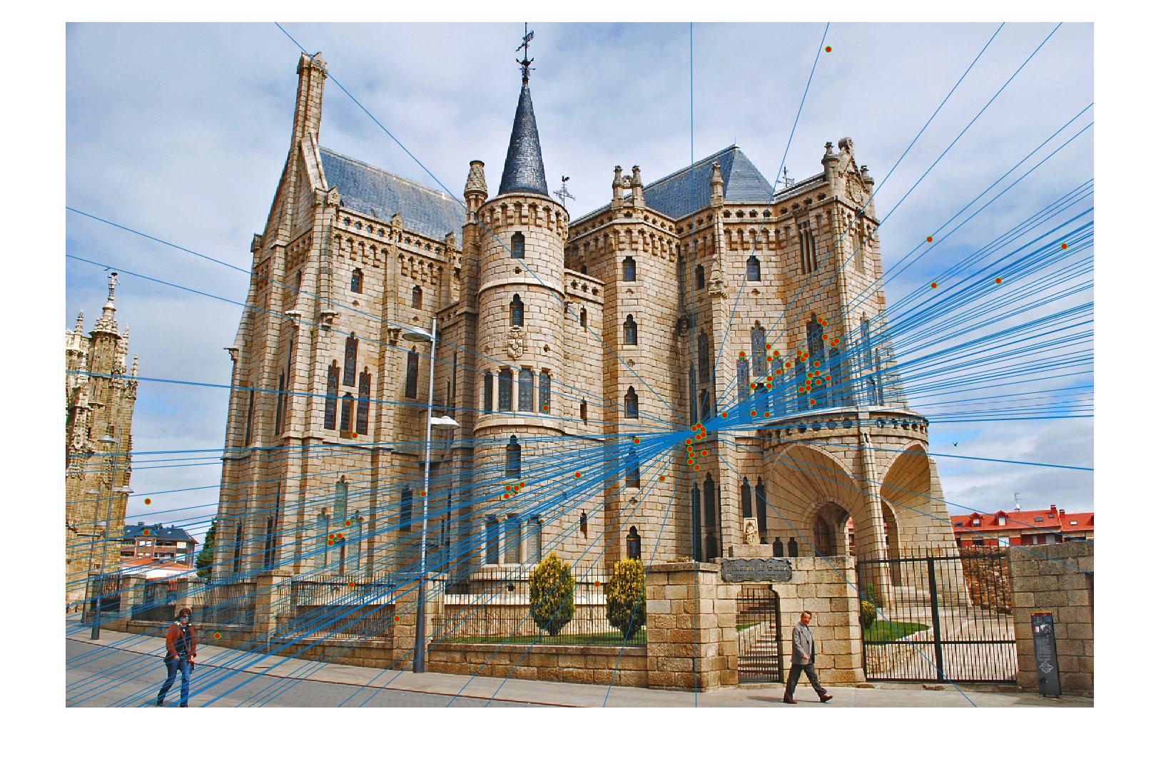
Here, we show a visualization of epipolar lines for the given pair of images.

Part III: Fundamental Matrix with RANSAC

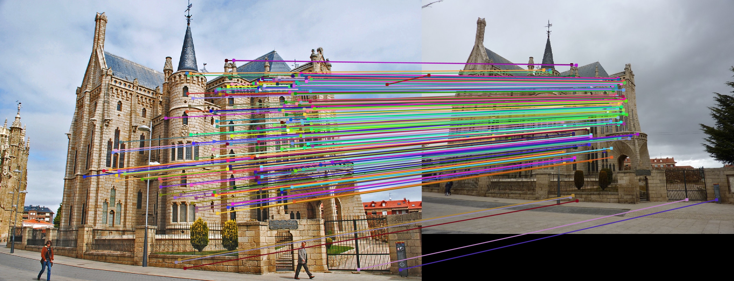
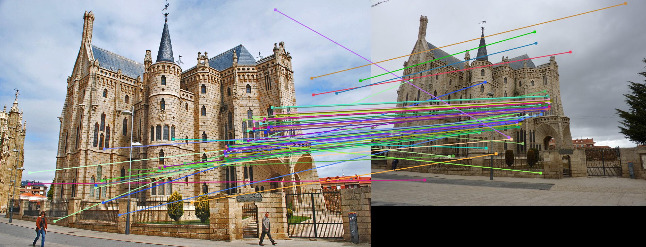
For two photographs of a scene it's unlikely that we would have perfect point corresponence with which to do the regression for the fundamental matrix. So, we compute the fundamental matrix with unreliable point correspondences computed with SIFT. Least squares regression is not appropriate in this scenario due to the presence of multiple outliers. In order to estimate the fundamental matrix from this noisy data, we need to use RANSAC in conjunction with fundamental matrix estimation.

We use VLFeat to do SIFT matching for image pairs. We use these putative point correspondences and RANSAC to find the "best" fundamental matrix. We iteratively choose some number of point correspondences (8 in this case), solve for the fundamental matrix, and then count the number of inliers. Inliers in this context are point correspondences that "agree" with the estimated fundamental matrix. In order to count how many inliers a fundamental matrix has, we use a distance metric based on the fundamental matrix. Here, we choose $\XFX'$ . We set the threshold between inliers and outliers as 0.001. Finally, we return the fundamental matrix with the most inliers

The expected number of iterations of RANSAC to find the "right" solution in the presence of outliers, N, is given by:

$N=\frac{log(1-p)}{log(1-(1-e)^s)}$

where e is the probability that a point is an outlier, s is the number of points in a sample, and p is the desired probability that we get a good sample. Here, we chose the following values of p, s and e which leads to ~10,000 iterations.

p = 0.3;
s = 8;
e = 0.7;
itr = round(log(1 - p) / log(1 - (1 - e)^s));

The relevant code snippet is shown below:

function [ Best_Fmatrix, inliers_a, inliers_b] = ransac_fundamental_matrix(matches_a, matches_b)

n_points = size(matches_a, 1);
matches_a = [matches_a ones(n_points, 1)];
matches_b = [matches_b ones(n_points, 1)];

p = 0.3;
s = 8;
e = 0.7;
itr = round(log(1 - p) / log(1 - (1 - e)^s));

matches = [];
for i = 1:itr
    idx = randperm(n_points, s);
    Fmatrix = estimate_fundamental_matrix(matches_a(idx, 1:2), matches_b(idx, 1:2));
    
    % diff = abs(diag(matches_b * Fmatrix * matches_a'));
    diff = abs(sum((matches_b * Fmatrix) .* matches_a, 2)); % Optimization
    matched_points = find(diff < 0.001);
    
    if (size(matched_points, 1) > size(matches, 1))
        matches = matched_points;
        Best_Fmatrix = Fmatrix;
    end
end

inliers_a = matches_a(matches, 1:2);
inliers_b = matches_b(matches, 1:2);

end

For many real images, the fundamental matrix that is estimated can be "wrong" (as in it implies a relationship between the cameras that must be wrong, e.g. an epipole in the center of one image when the cameras actually have a large translation parallel to the image plane). The estimated fundamental matrix can be wrong because the points are coplanar or because the cameras are not actually pinhole cameras and have lens distortions. This happens more often without normalization.

Results

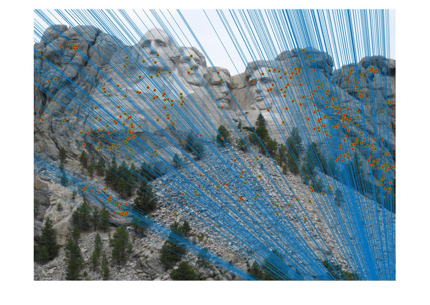
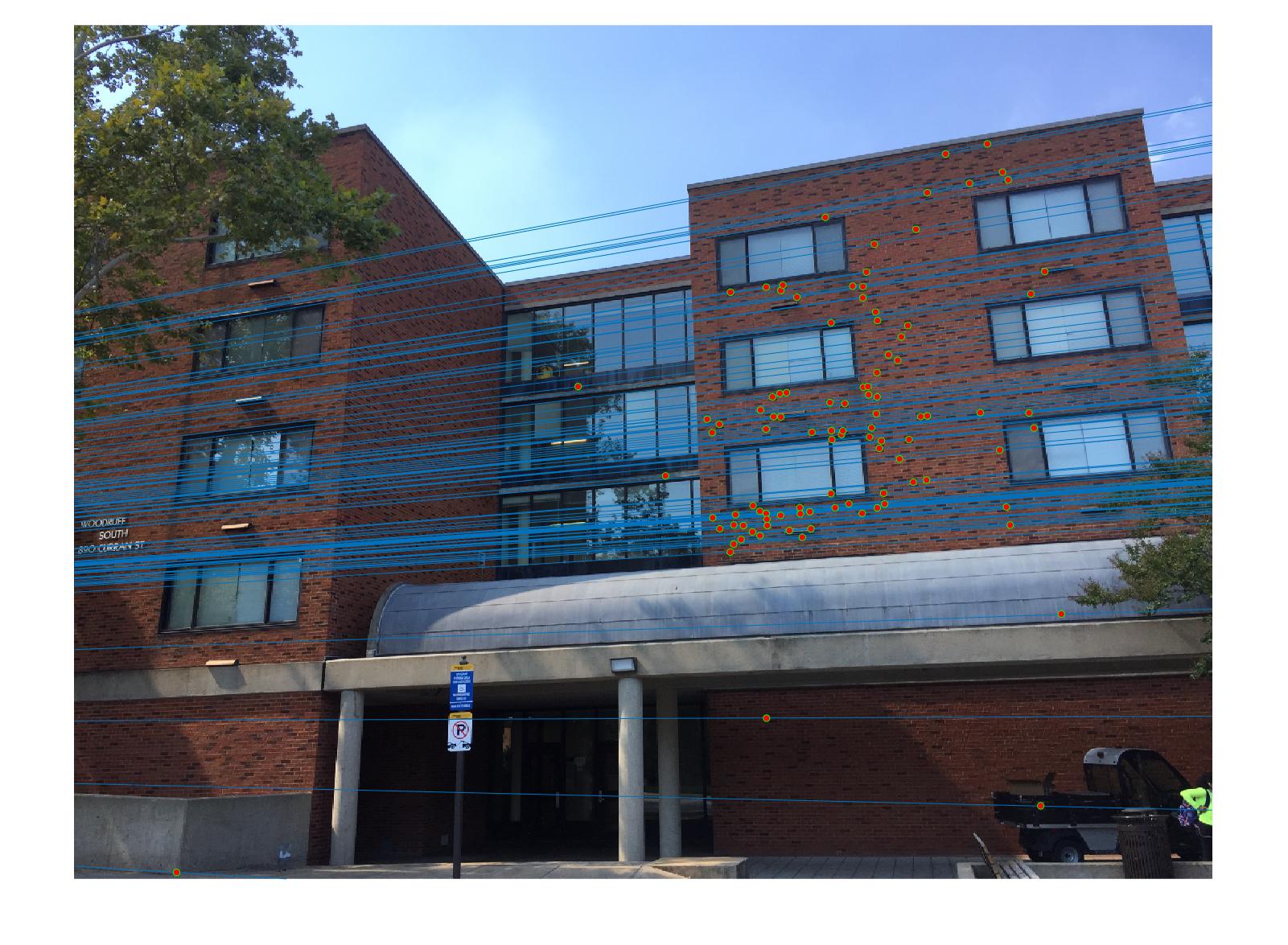
Note that these results are with normalization. The effect of normalization is demonstrated in the next section. The RANSAC algorithm seems to do well for all pairs of images with normalization and the selected hyperparameters. We also mention the number of inliers for each pair of images with the given hyperparameters.

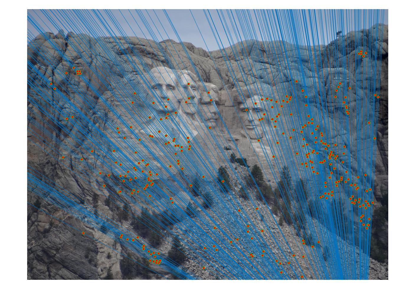
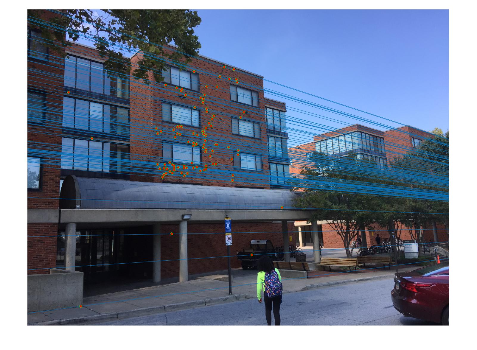
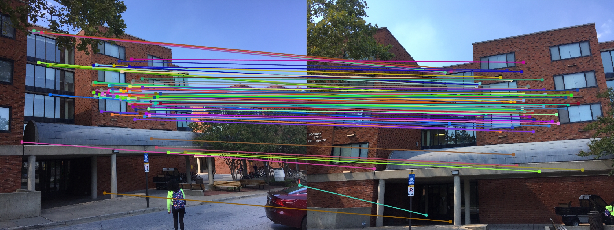
Mt. Rushmore (319 inliers)

Woodruff Hall (122 inliers)

Extra Credit

Normalization

The fundamental matrix estimate can be improved by normalizing the coordinates before computing the fundamental matrix. Typically, we perform normalization through linear transformations as described below to make the mean of the points zero and the average magnitude about 1.0 or some other small number (square root of 2 is also recommended).

$\begin{pmatrix}u' & v' & 1 \end{pmatrix} = \begin{pmatrix}s & 0 & 0 \\ 0 & s & 0 \\ 0 & 0 & 1 \end{pmatrix} \begin{pmatrix}1 & 0 & -c_u \\ 0 & 1 & -c_v \\ 0 & 0 & 1 \end{pmatrix} \begin{pmatrix}u \\ v \\ 1 \end{pmatrix}$

The transform matrix T is the product of the scale and offset matrices. $\c_u$ and $\c_v$ are the mean coordinates. To compute a scale s you could estimate the standard deviation after substracting the means. Here, we scale the coordinates such that the average squared distance from the origin (after centering) is 2. We use different scale matrices for the two images.

We also need to use the scaling matrices to adjust the fundamental matrix so that it can operate on the original pixel coordiantes as follows:

$F_{orig} = T_{b}^{T} * F_{norm} * T_{a}$

The relevant code snippet is shown below:

function [ T ] = get_normalization_matrix(points)

    center = mean(points);
    mean_dist = sqrt(mean(sum(bsxfun(@minus, points, center) .^2, 2)));
    scale = sqrt(2) / mean_dist;
    T = [scale    0    -scale*center(1);
           0    scale  -scale*center(2);
           0      0           1         ];
% No normalization
%    T = eye(3);
end

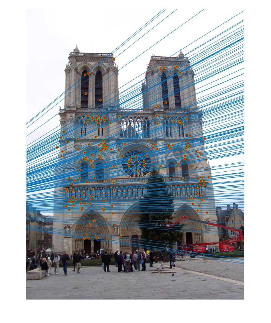
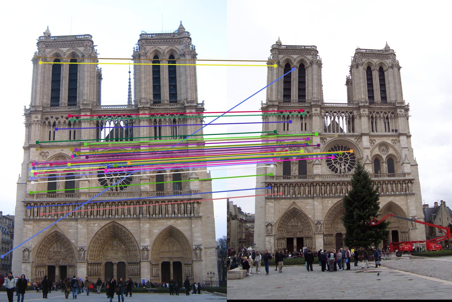
Normalization is necessary for Episcopal Gaudi and Notre Dame and greatly improves results. While the improvement is not that drastic for other pairs of image, normalization still improves results significantly. We also notice that the number of inliers falls drastically without normalization.

Notre Dame with normalization (171 inliers)

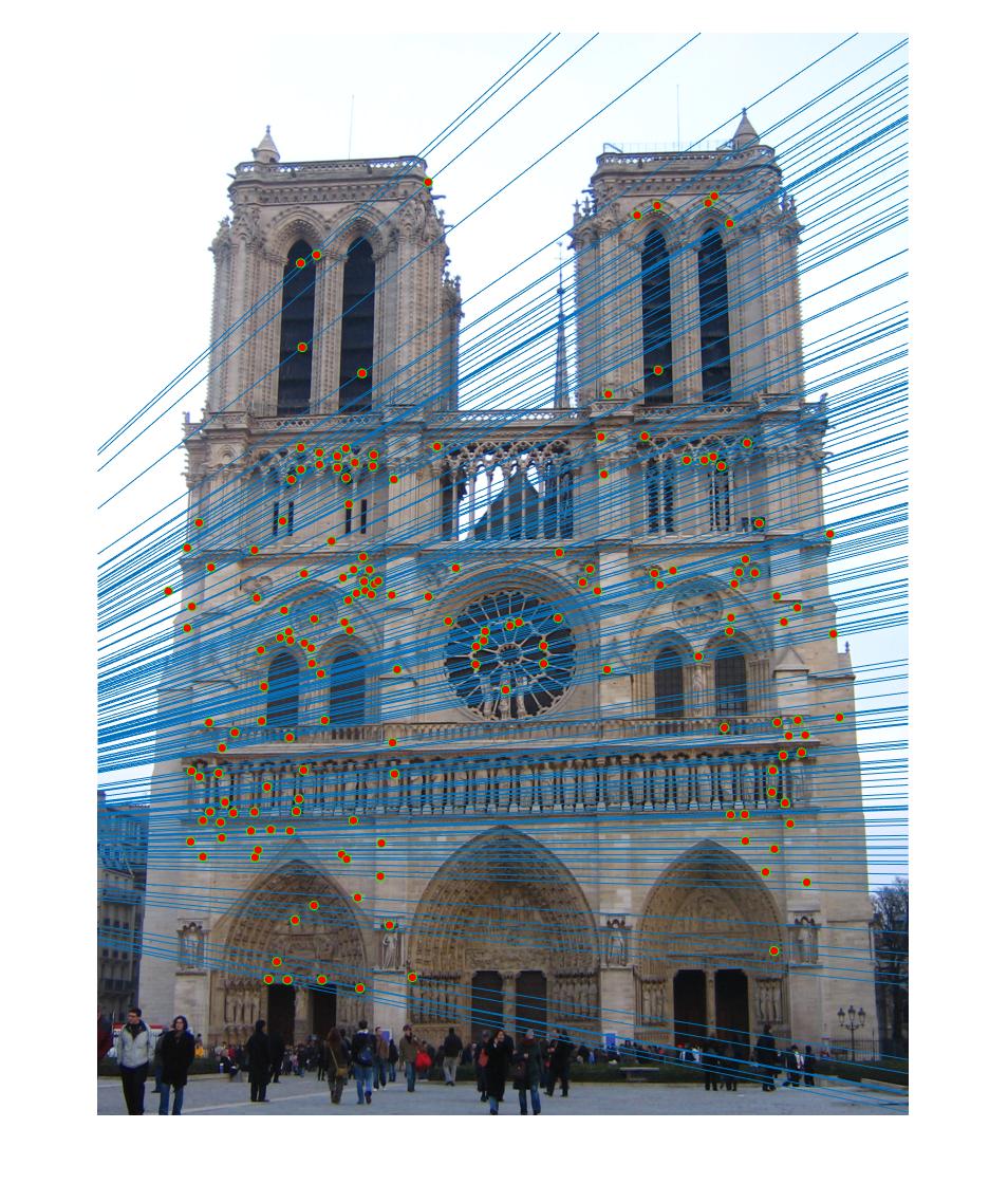
Notre Dame without normalization (45 inliers)

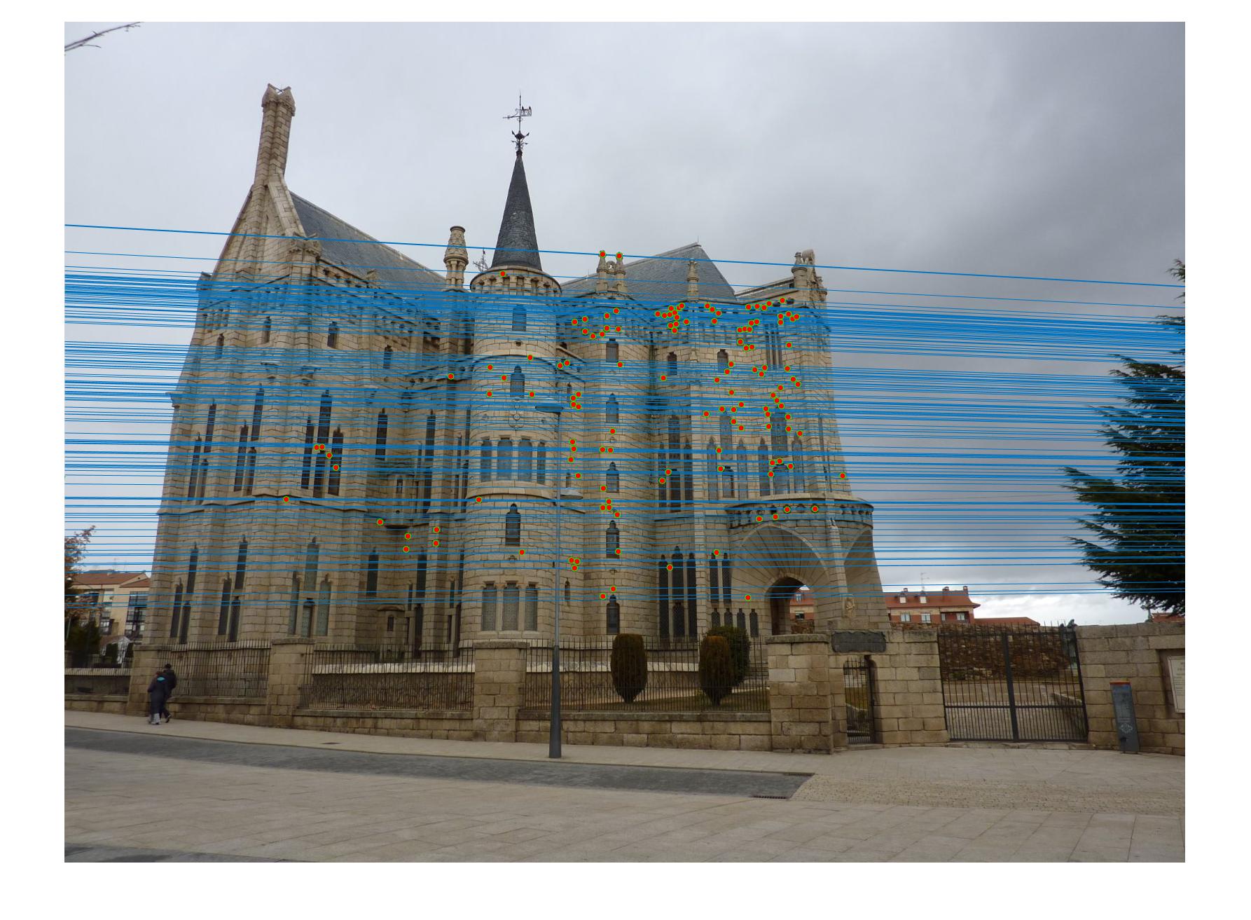
Episcopal Gaudi with normalization (120 inliers)

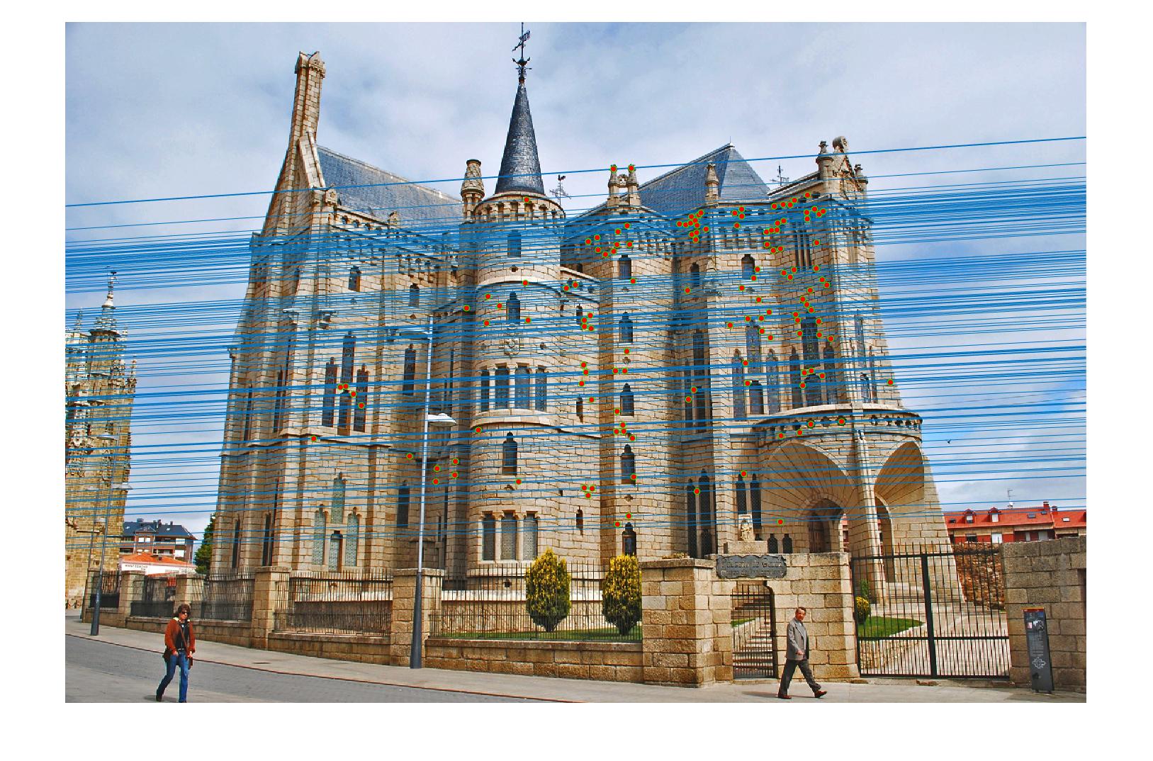
Episcopal Gaudi without normalization (71 inliers)

Optimization

The code has been optimized for speed and vectorized wherever possible. Another key optimization is inside the RANSAC loop when we are evaluatiing whether points are inliers. There are multiple ways to do this. We need to find $\XFX'$ for each pair of points. We can do this either in a for loop or by using matrix multiplication. The matrix multiplication computes this for all points at once. However, we notice that we only need the diagonal of the resulting matrix. So, the calculation time can be reduced to O(n) instead of O(n^2) for the second multiplication. Implementing this gives us a runtime of ~4 seconds compared to ~45 seconds for the full matrix multiply for a roughly 10x speedup.

The relevant code snippet is shown below:

function [ Best_Fmatrix, inliers_a, inliers_b] = ransac_fundamental_matrix(matches_a, matches_b)

...

for i = 1:itr
    ...
    % diff = abs(diag(matches_b * Fmatrix * matches_a')); % O(n^2)
    diff = abs(sum((matches_b * Fmatrix) .* matches_a, 2)); % O(n)
    ...
end

...

end

Shaswat Shah

Project 3: Camera Calibration and Fundamental Matrix Estimation with RANSAC

Overview

Part I: Camera Projection Matrix

Part II: Fundamental Matrix Estimation

Part III: Fundamental Matrix with RANSAC

Results

Mt. Rushmore (319 inliers)

Woodruff Hall (122 inliers)

Extra Credit

Normalization

Notre Dame with normalization (171 inliers)

Notre Dame without normalization (45 inliers)

Episcopal Gaudi with normalization (120 inliers)

Episcopal Gaudi without normalization (71 inliers)

Optimization