Project 3 / Camera Calibration and Fundamental Matrix Estimation with RANSAC
This project involved estimating the camera projection matrix (maps 3D world coordinates to image coordinates), and the fundamental matrix (relates points in one scene to epipolar lines in another).
Part I. Camera Projection Matrix
For moving from 3D world coordinates to 2D camera coordinates, we can utilize this equation:
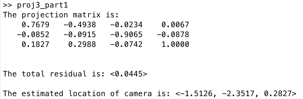
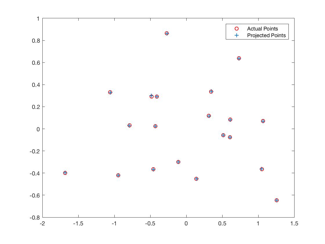
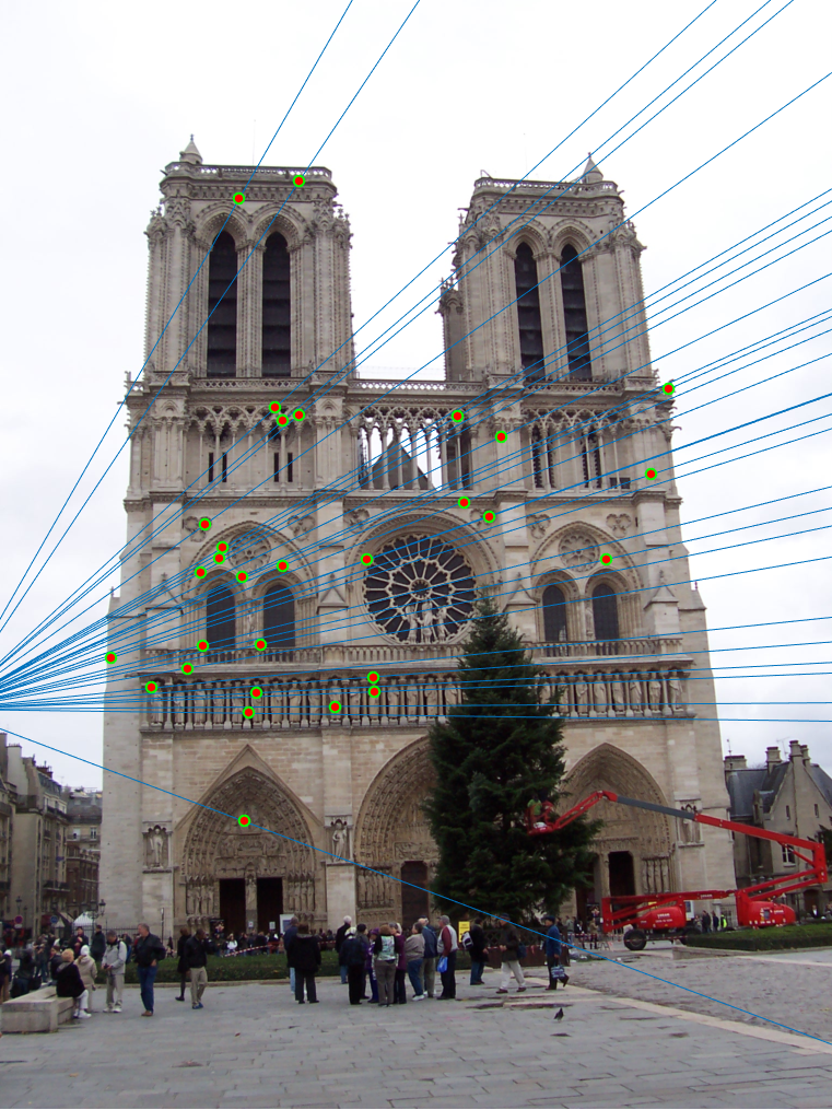
I constrained the last value (m_34) to 1 (to fix a scale), and then solved it using least squares in MATLAB. Here are my results -
MATLAB Code for Camera Projection Matrix
							[size_2d, ~] = size(Points_2D);
							A = zeros(2 * size_2d, 11); % constrain last value for scaling
							B = zeros(2 * size_2d, 1);

							u = Points_2D(:,1);
							v = Points_2D(:,2);
							X = Points_3D(:,1);
							Y = Points_3D(:,2);
							Z = Points_3D(:,3);

							for i = 1:size_2d
							    j = 2 * i;
							    A(j - 1, :) = [X(i), Y(i), Z(i), 1, 0, 0, 0, 0, ...
							                   -u(i)*X(i), -u(i)*Y(i), -u(i)*Z(i)];
							    A(j, :)     = [0, 0, 0, 0, X(i), Y(i), Z(i), 1, ...
							                   -v(i)*X(i), -v(i)*Y(i), -v(i)*Z(i)];
							    B(j -1, 1)  = u(i);
							    B(j, 1)     = v(i);
							end

							% least-squares
							M_init = transpose([A\B; 1]);
							M = [M_init(1:4); M_init(5:8); M_init(9:12)]; % reshape
MATLAB Code for Camera Center
							% Let us define M as being made up of a 3x3 we'll call Q
							% and a 4th column will call m4 :
							Q = M(1:3, 1:3);
							m4 = M(1:3, 4);

							Center = -inv(Q) * m4; % from class
Part II. Fundamental Matrix Estimation
The Fundamental Matrix: 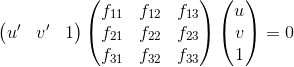
Steps to Estimate:
						 8-point algorithm
						 1. Solve a system of homogeneous linear equations
						   a. Write down the system of equations
						       uu'f11 + uv'f12 + uf13  + vu'f21 + vv'f22 + ...
						       vf23   + u'f31  + v'f32 + f33    = 0
						   b. Solve f from Af=0 using SVD
						       [U, S, V] = svd(A);
						       f = V(:, end);
						       F = reshape(f, [3 3])`;
						 2. Resolve det(F) = 0 constraint by SVD
						       [U, S, V] = svd(F);
						       S(3,3) = 0;
						       F = U*S*V`;
|
MATLAB Code for Estimating Fundamental Matrix
							[sizeA, ~] = size(Points_a);
							[sizeB, ~] = size(Points_b);

							A = zeros(sizeA, 9);
							u = Points_a(:,1);
							v = Points_a(:,2);
							u1 = Points_b(:,1);
							v1 = Points_b(:,2);

							for i = 1:sizeA
							    A(i, :) = [u(i) * u1(i), v(i) * u1(i), u1(i), u(i) * v1(i), ...
							               v(i) * v1(i), v1(i), u(i), v(i), 1];
							end


							[U, S, V] = svd(A);
							f = V(:, end);
							F_matrix = reshape(f, [3 3])`;

							[U, S, V] = svd(F_matrix);
							S(3,3) = 0;
							F_matrix = U*S*V`;
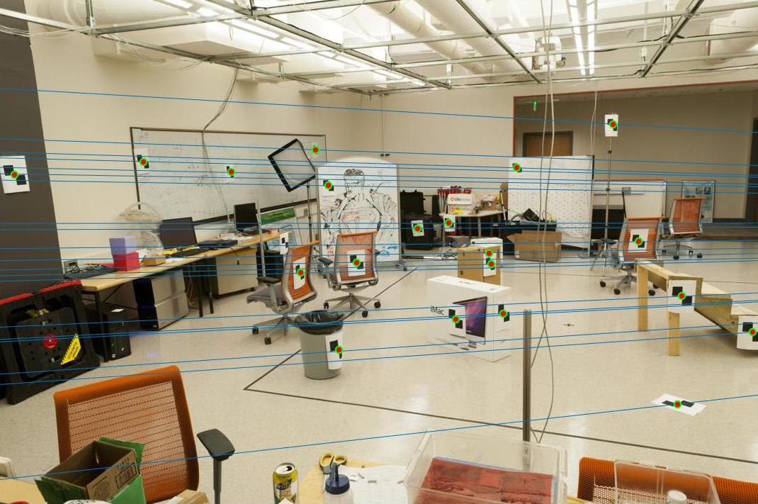
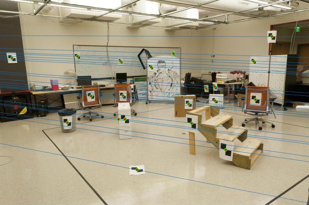
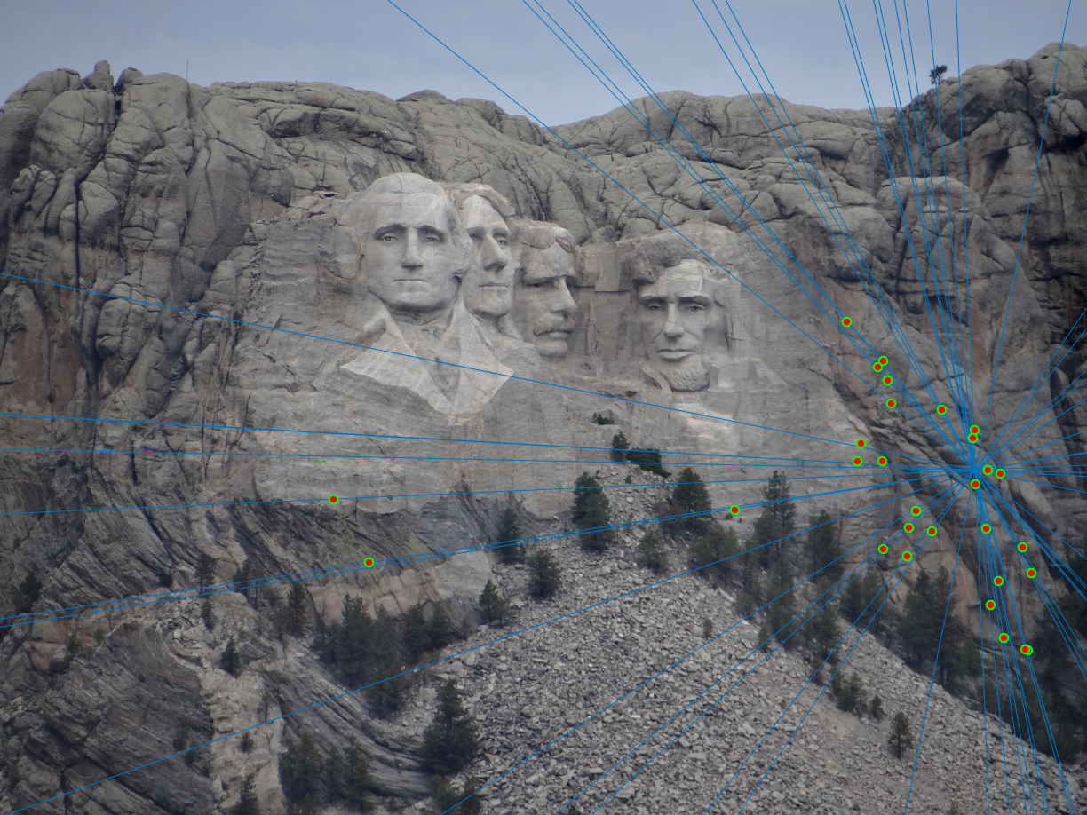
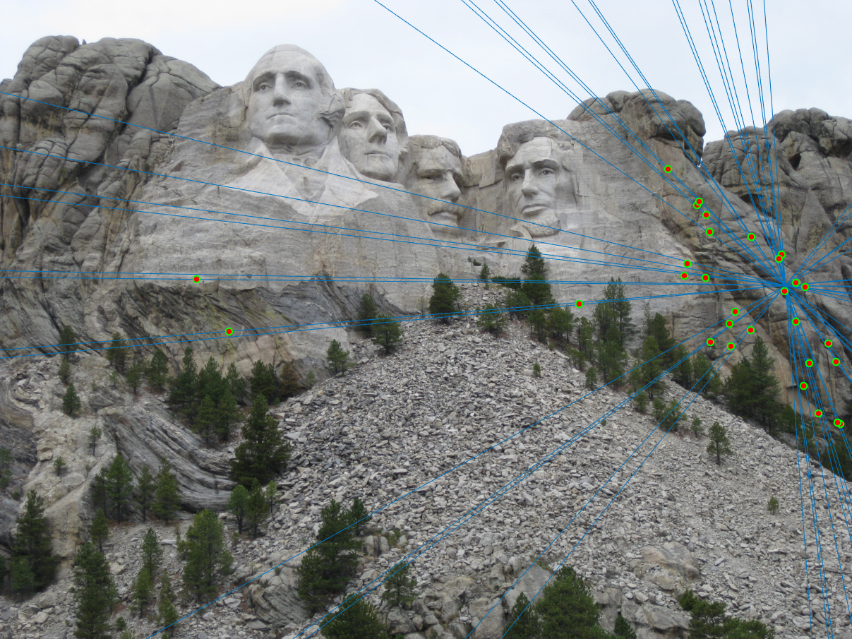
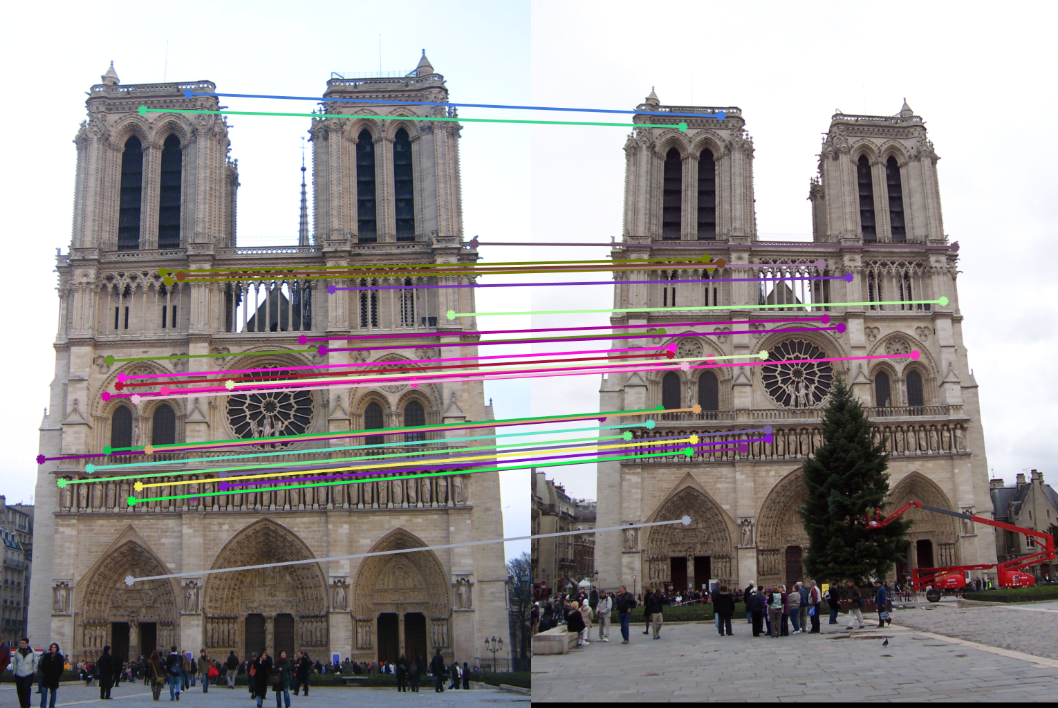
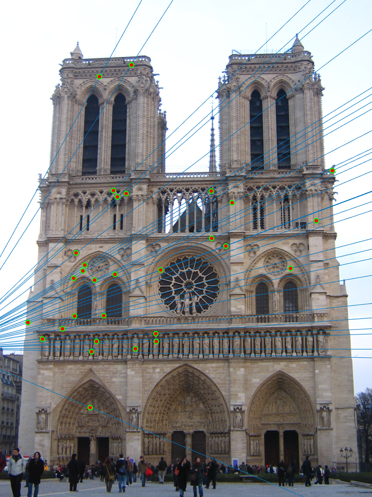
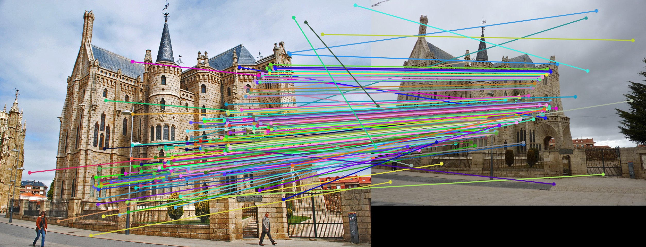
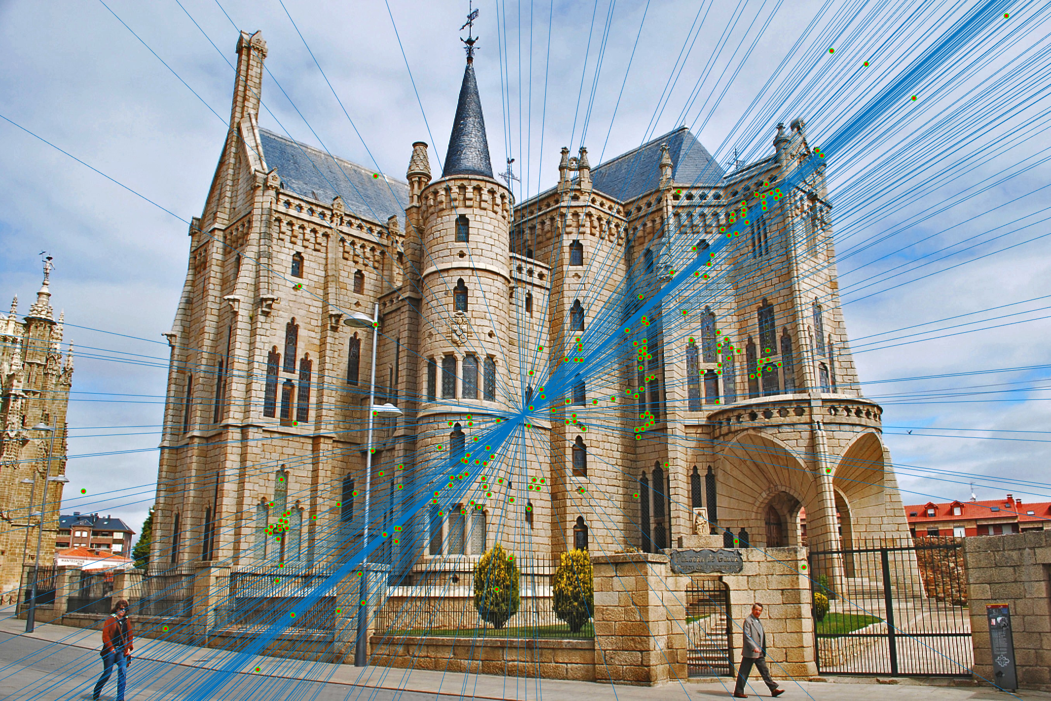
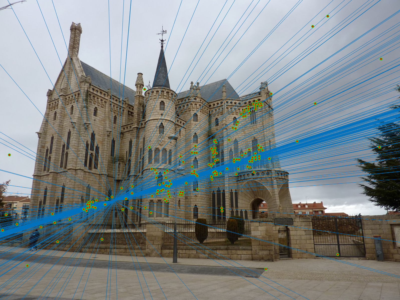
Part III. Fundamental Matrix with RANSAC
Point correspondences computed with SIFT are unreliable and noisy. Using least squares to solve for the fundamental matrix will not work well. However, RANSAC is suitable when multiple outliers are present. It has 3 steps -
- Sample (randomly) the number of points required to fit the model
- Solve for model parameters using samples
- Score by the fraction of inliers within a preset threshold of the model
The results:
For the Mt. Rushmore and Notre Dame images, 30 inliers are randomly chosen to be displayed for a cleaner visualization.
|
|
|
|
|
|
MATLAB Code for Estimating Fundamental Matrix with RANSAC
							num_iterations = 1500; % > 1177
							threshold = 0.005;
							best_num_inliers = 0;

							num_elems = size(matches_a, 1);

							for i = 1:num_iterations
							    rand_indices = randperm(num_elems, 8);
							    rand_a = matches_a(rand_indices, :);
							    rand_b = matches_b(rand_indices, :);
							    F_matrix = estimate_fundamental_matrix(rand_a, rand_b);

							    a_inliers = [];
							    b_inliers = [];
							    num_inliers = 0;
							    for n = 1 : num_elems
							        error = [matches_b(n, :) 1] * F_matrix * [matches_a(n, :) 1]';
							        if abs(error) < threshold
							            a_inliers(end+1, :) = matches_a(n, :);
							            b_inliers(end+1, :) = matches_b(n, :);
							            num_inliers = num_inliers + 1;
							        end
							    end
							    if num_inliers > best_num_inliers
							        best_num_inliers = num_inliers;
							        inliers_a = a_inliers;
							        inliers_b = b_inliers;
							        Best_Fmatrix = F_matrix;
							    end
							end