Project 3 / Camera Calibration and Fundamental Matrix Estimation with RANSAC
This project is an introduction to Camera and Scene geometry. It is made of three parts:
- Computing the Camera Projection Matrix
- Estimation of the Fundamental Matrix
- Fundamental Matrix using RANSAC
Camera Projection Matrix
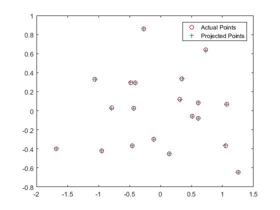
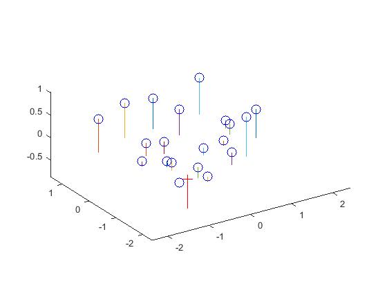
Here, a projection matrix that maps the 3D world coordinates to 2D Image coordinates is computed. The M matrix is set up from the system of homogeneous equations, and it is solved using Singular Value Decomposition. A particular camera parameter, the Camera center is extracted from this matrix.
The camera center is found to be at <-1.5127, -2.3517, 0.2826>
Code
The Matlab code to find theCamera Projection Matrix is shown below.
h=1;

for k = 1:size(Points_2D,1)
    A(h,:) = [Points_3D(k,1) Points_3D(k,2) Points_3D(k,3)...
              1 0 0 0 0 ...
             -Points_2D(k,1)*Points_3D(k,1) -Points_2D(k,1)*Points_3D(k,2)...
             -Points_2D(k,1)*Points_3D(k,3) -Points_2D(k,1)];
    A(h+1,:) = [0 0 0 0 Points_3D(k,1) ...
              Points_3D(k,2) Points_3D(k,3) 1 ...
             -Points_2D(k,2)*Points_3D(k,1) -Points_2D(k,2)*Points_3D(k,2)...
             -Points_2D(k,2)*Points_3D(k,3) -Points_2D(k,2)];
    h= h+2;
end
[~, ~, V] = svd(A);
M = -reshape(V(:, end), 4, 3)';
Camera Center is shown below.
Q = M(:,1:3);
m4 = M(:,4);
Center = -inv(Q)*m4;
Results
|
Estimation of Fundamental Matrix
Here, a fundamental matrix which maps the points in one image to lines in another is computed. The method followed is similar to the one above, by solving a system of homogeneous equations using Matlab's svd command.
Code
The Matlab code to find theFundamental Matrix is shown below.
for idx = 1: size(Points_a,1)
 A(idx,:) = [...
    Points_a(idx,1)*Points_b(idx,1) Points_a(idx,2)*Points_b(idx,1) Points_b(idx,1)...
    Points_a(idx,1)*Points_b(idx,2) Points_a(idx,2)*Points_b(idx,2) Points_b(idx,2)...
    Points_a(idx,1) Points_a(idx,2) 1];
end
[U, S, V] = svd(A);
f = V(:, end);
F_matrix = reshape(f, [3 3])';

[U, S, V] = svd(F_matrix);
S(3,3) = 0;
F_matrix = U*S*V';
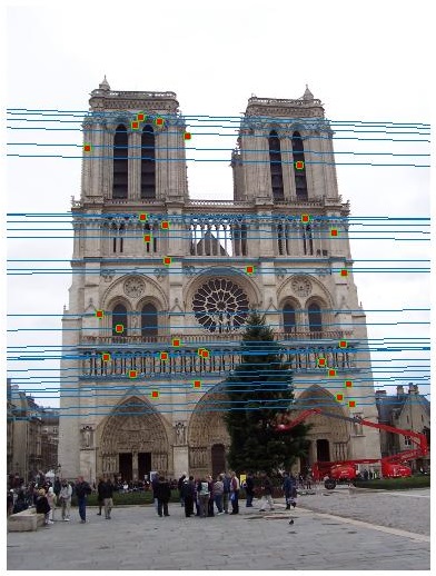
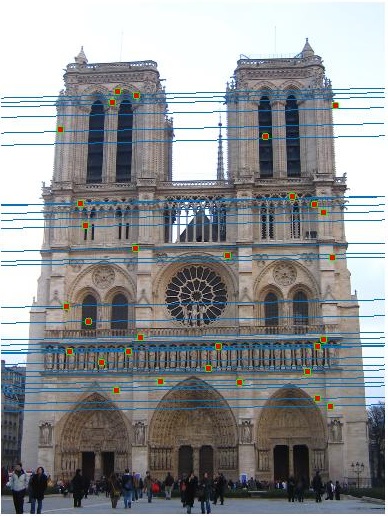
Results
A nearly perfect result is obtained here, as the points correspond to the ground truth data.
With the addition of noise, the results tend to get swayed.
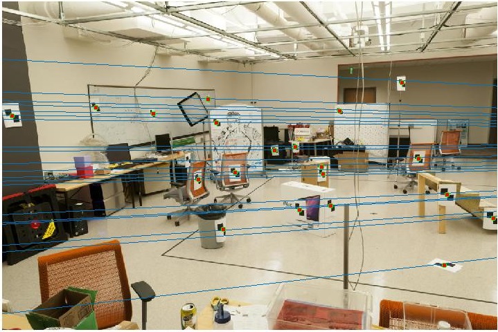
Fundamental Matrix using RANSAC
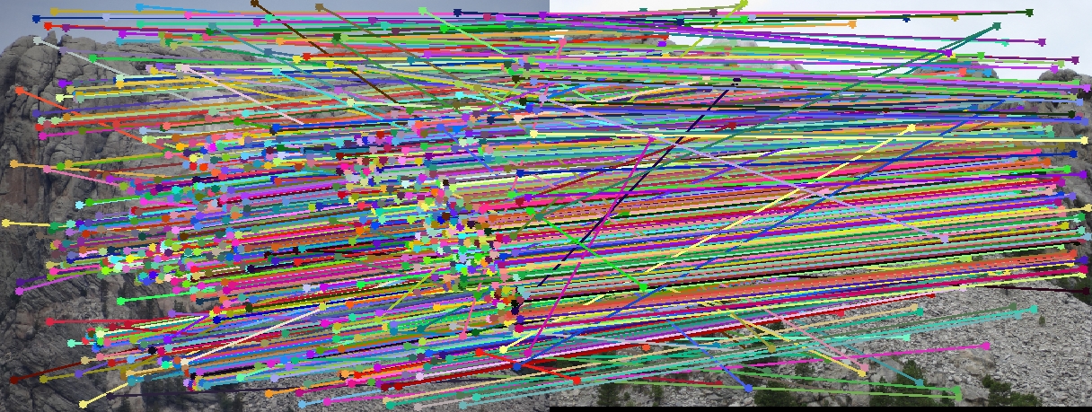
Unreliable correspondences are found between the two images using VLFeat for SIFT matching. From these, the fundamental matrix is estimated using RANSAC.
8 pairs of random correspondences are chosen iteratively, and the fundamental matrix is computed for each of them. The total number of inliers which agree with the computed fundamental matrix is counted.
The matrix with the largest number of inliers becomes the fundamental matrix for the given set of equations.
Here, 30 matches are chosen randomly for visualization
Code
The Matlab code to estimate theFundamental Matrix using RANSAC is shown below.
matches_num = size(matches_a,1);
in_max = 0;
thresh = 0.05;
for iter = 1:1000
    %Sample (randomly) the number of points required to fit the model
    sample_idx = randsample(matches_num,8);
    sample_a  = matches_a(sample_idx, :);
    sample_b = matches_b(sample_idx, :);

    %Estimate fundamental matrix
    F_matrix = estimate_fundamental_matrix(sample_a, sample_b);
    in_a = [];
    in_b = [];
    in_num = 0;
    %Solve for model parameters using samples
    for n = 1:matches_num
        error = [matches_a(n,:) 1]*F_matrix'*[matches_b(n,:) 1]';
        if abs(error) < thresh
            in_a(end+1,:) = matches_a(n,:);
            in_b(end+1,:) = matches_b(n,:);
            in_num = in_num + 1;
        end
    end

    %Score by the fraction of inliers within a preset threshold of the model
    if in_num > in_max
        in_max = in_num;
        Best_Fmatrix = F_matrix;
        inliers_a = in_a;
        inliers_b = in_b;
    end
end

%Take 30 random samples for visualization
idx = randsample(size(inliers_a,1),30);
inliers_a = inliers_a(idx,:);
inliers_b = inliers_b(idx,:);
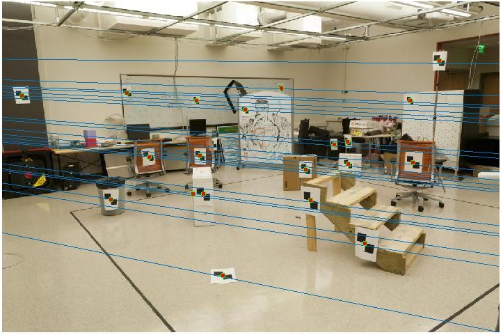
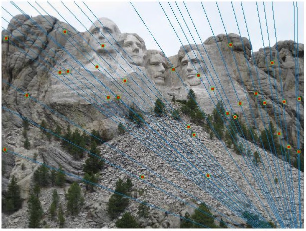
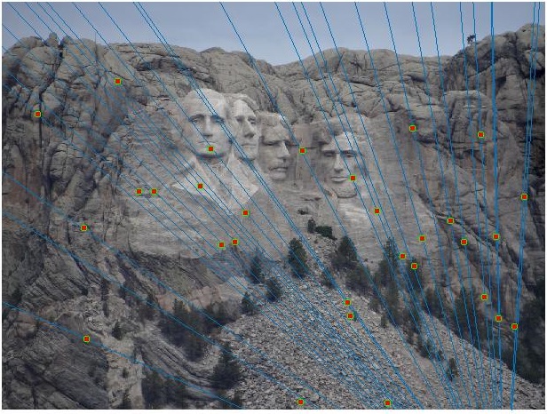
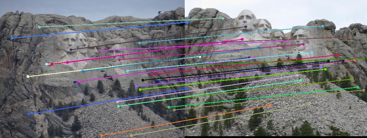
Results
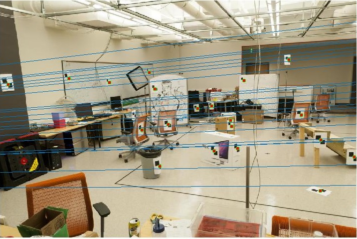
Mount Rushmore Image Pair
Visualizationof all the SIFT features
Notre Dame Image Pair
Graduate Credit - Normalization of Fundamental Matrix
To achieve better results, the fundamental matrix is normalised. The accuracy of the matching increases significantly due to normalization.
The centroid is calculated and the mean distance to the centroid is calculated using the following formulae

The normalization vectors are then found, and multiplied with the Fundamental matrix

Code
The Matlab code to find theFundamental Matrix is shown below.
num = size(Points_a,1);
B = -ones(num,1);

%Calculaye the centroid
a_u = sum(Points_a(:,1))/num;
a_v = sum(Points_a(:,2))/num;
b_u = sum(Points_b(:,1))/num;
b_v = sum(Points_b(:,2))/num;

%Calculate the distance from centroid
d_a = num/sum(((Points_a(:,1)-a_u).^2 + (Points_a(:,2)-a_v).^2).^(1/2));
d_b = num/sum(((Points_b(:,1)-b_u).^2 + (Points_b(:,2)-b_v).^2).^(1/2));

%Normalization vector
T_a = [d_a 0 -a_u*d_a; 0 d_a -d_a*a_v; 0 0 1];
T_b = [d_b 0 -b_u*d_b; 0 d_b -d_b*b_u; 0 0 1];

%Normalized points
Points_a = T_a*[Points_a ones(num,1)]';
Points_a = Points_a';
Points_b = T_b*[Points_b ones(num,1)]';
Points_b = Points_b';

%Calculation of matrix from system equations
for idx = 1: size(Points_a,1)
A(idx,:) = [...
    Points_a(idx,1)*Points_b(idx,1) Points_a(idx,2)*Points_b(idx,1) Points_b(idx,1)...
    Points_a(idx,1)*Points_b(idx,2) Points_a(idx,2)*Points_b(idx,2) Points_b(idx,2)...
    Points_a(idx,1) Points_a(idx,2)];
end

%Solving the A matrix
F_matrix = A\B;
F_matrix = [F_matrix;1];
F_matrix = reshape(F_matrix,[3 3]);

%Normalized Funadamental matrix
F_matrix = T_a'*F_matrix*T_b;
F_matrix = F_matrix';

%Resolve det(F) = 0
[U, S, V] = svd(F_matrix);
S(3,3) = 0;
F_matrix = U*S*V';
Results
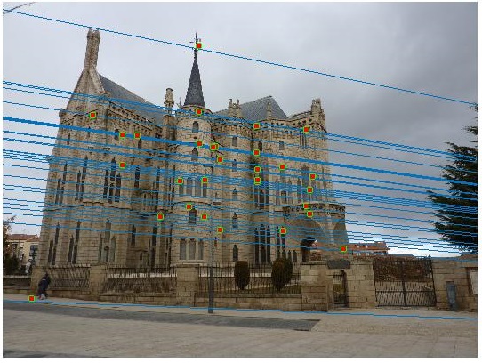
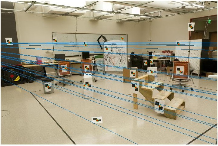
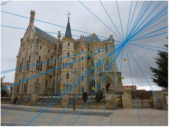
Episcopal Gaudi Image Pair - Before Normalization
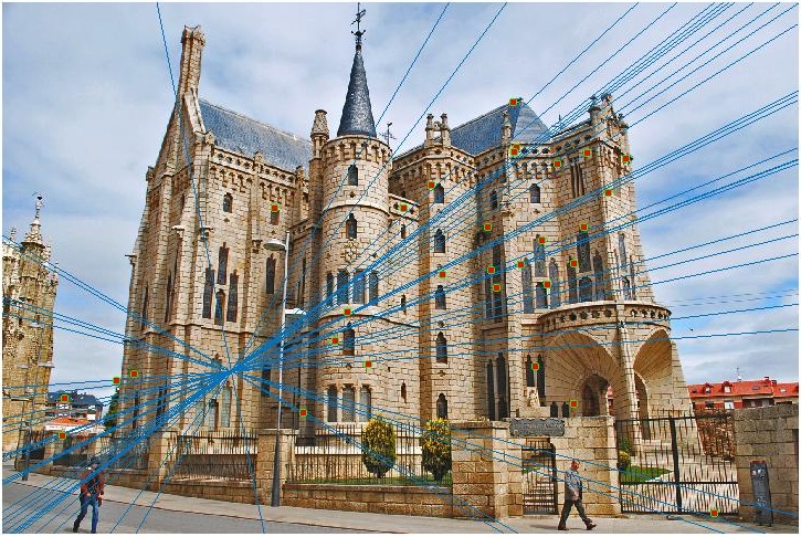
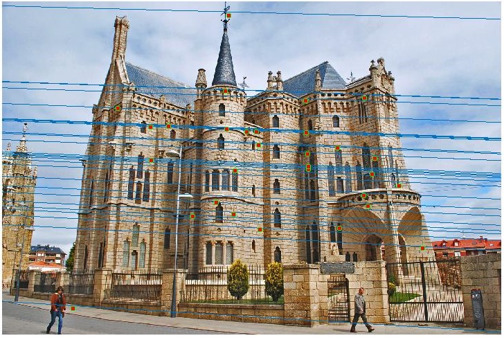
Episcopal Gaudi Image Pair - After Normalization