Project 3 / Camera Calibration and Fundamental Matrix Estimation with RANSAC
Part 1 Projection Matrix
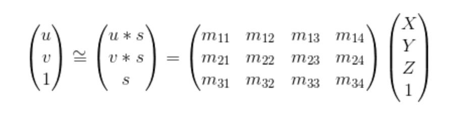
Fig 1.0
The function in Figure 1.0 is the function that was used to caculate the projection matrix. It can be reduced to a mutiplication between 2 matrices. We can then get the projection matrix by solving the linear regression and scaling it with singular value decompoistion (SVD). I composed the matrix by puting the following code in a for loop.
    X = Points_3D(n, 1);
    Y = Points_3D(n, 2);
    Z = Points_3D(n, 3);
    u = Points_2D(n, 1);
    v = Points_2D(n, 2);
    R(2*n-1:2*n, :) = [X Y Z 1 0 0 0 0 -u*X -u*Y -u*Z -u;
        0 0 0 0 X Y Z 1 -v*X -v*Y -v*Z -v];
	[U,S,V] = svd(R, 0);
	M = -1 * V(:,end);

	M = reshape(M,[], 3)';
Part 2 Fundamental Matrix
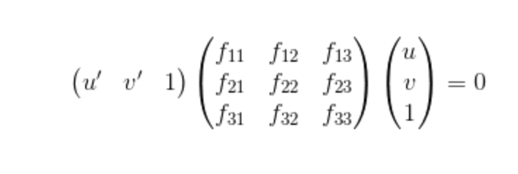
Fig 2.0
The function in Figure 2.0 is the function we used to caculate the fundamental matrix. The fundamental matrix is a 3x3 matrix that represents relations in stereo images. In epipolar geometry where there is a pair of points x and x', Fx represents a line that the corresponding point x' must lie on. This means that (x^T)Fx' must equal 0. This is how the error will be caculated in part 3 (RANSAC). The following code is how the matrices for linear regression and SVD are set up.
   u = Points_b(n, 1);
   v = Points_b(n, 2);
   u_prime = Points_a(n, 1);
   v_prime = Points_a(n, 2);
   A(n, :) = [u*u_prime u*v_prime u v*u_prime v*v_prime v u_prime v_prime 1];
	[U,S,V] = svd(A);
	f = V(:,end);
	F = reshape(f,[3 3])';

	[U,S,V] = svd(F);
	S(3,3) = 0;
	F_matrix = U*S*V';
Part 3 RANSAC
There are 3 parts to RANSAC (Random Sample Consensus). The first part is randomly sample a set amount of points in the matched points that were dicovered by SIFT. Here is the code:
	points_a = [];
	points_b = [];
	rand = randsample(size(matches_a,1), s);
	for j= 1:s
		points_a = [points_a; matches_a(rand(j),:)];
		points_b = [points_b; matches_b(rand(j),:)];
	end
Then you find the fundamental matrix with the selected points
The third part uses the fundamental matrix to estimate inliers and outliers for all points. The best model will be the fundamental matrix that includes the most inliers.
	for k = 1:size(matches_a, 1)
		x = [ matches_a(k, :) 1 ].';
		x_prime = [ matches_b(k, :) 1];
		error = abs(x_prime * f_matrix * x);
		if error < thres
			a = [a; matches_a(k, :)];
			b = [b; matches_b(k, :)];
		end
	end

	if size(a,1) > max
		inliers_a = a;
		inliers_b = b;
		max = size(inliers_a,1);
		Best_Fmatrix = f_matrix;
	end
Results
Mount Rushmore (N = 1500, Samples = 20, Thershold = 0.005)
.jpg)
-1.jpg)
-2.jpg)
|
Mount Rushmore (N = 1500, Samples = 20, Thershold = 0.001)
.jpg)
-1.jpg)
-2.jpg)
|
Notre Dame (N = 1500, Samples = 20, Threshold = 0.001)
.jpg)
-1.jpg)
-2.jpg)
|
Woodies (N = 150, Samples = 10, Threshold = 0.005)
.jpg)
-1.jpg)
-2.jpg)
|
Woodies (N = 300, Samples = 10, Threshold = 0.005)
.jpg)
-1.jpg)
-2.jpg)
|
Woodies (N = 1500, Samples = 20, Threshold = 0.001)
.jpg)
-1.jpg)
-2.jpg)
|
With the woodies exaples you can clearly see how the threshold can alter the outcome of the fitting, it seems like the impact of setting a lower threshold has a larger impact than changing the number of iterations.