Project 3 : Camera Calibration and Fundamental Matrix Estimation with RANSAC
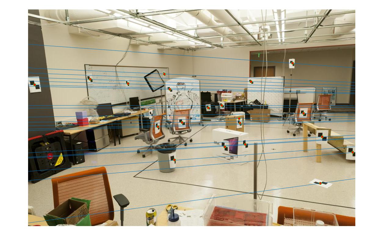
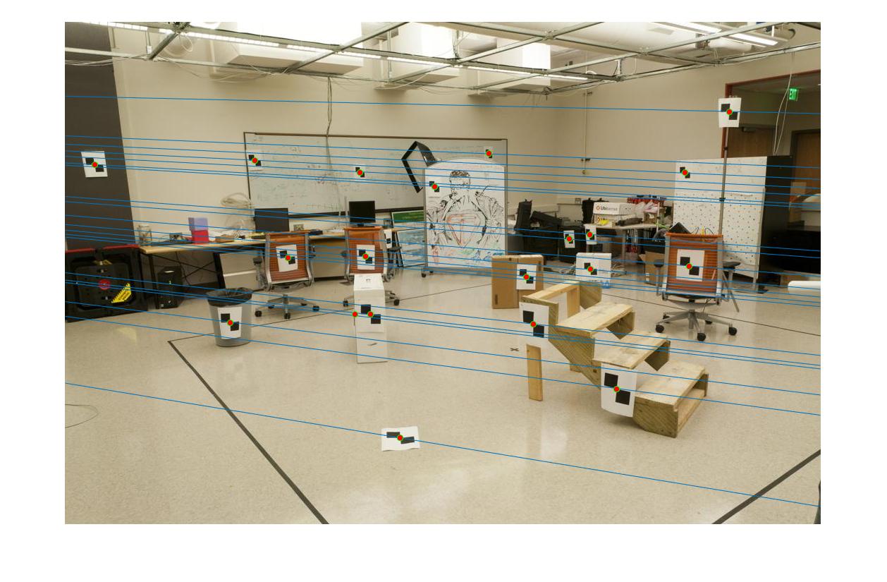
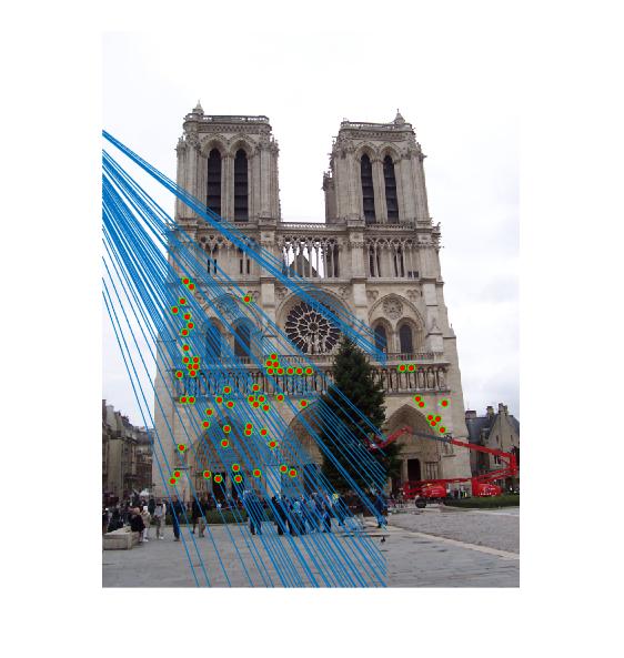
Epipolar lines for a pair of images |
The project aims at being able to caliberate the camera, creating robust fundamental matrix and implementing RANSAC. The first part aims at being able to detect the position of the camera using concept of fundamental matrix. Second part of project focuses on finding fundamental matrix. The fundamental matrix obtained using the algorithm in second part has some noise and thus, the third part aims at using RANSAC algorithm to remove noise (i.e outliers) and obtain a robust fundamental matrix. The can be listed as:
- Camera Calibration and finding camera centre.
- Calculate fundamental matrix.
- RANSAC Algorithm for robust fundamental matrix.
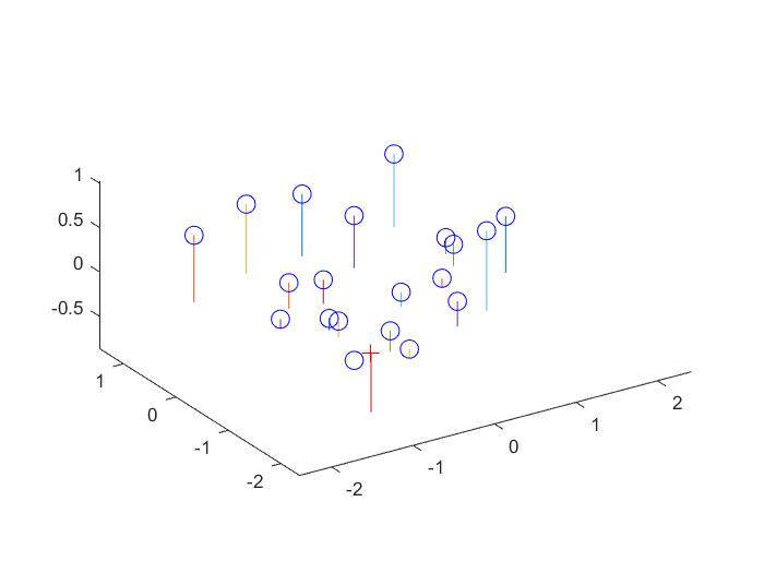
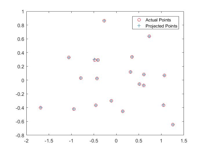
For calibrating the camera, we need to find know a location of few points in image plane and their corresponding location in real world. Using this data we get linear regression equation. It is of form [x y 1] = M*[x y z 1], where M is the projection matrix. The matrix M can have different values depending on the scale and thus can result in many different solutions. To overcome this part, we fix the last element M(3,4) to 1. This enables us to calculate the projection matrix. It basically denotes the relation between the 3D points in world and 2D points in the image.
The projection matrix obtained for our data points:
| -0.4583 | ааа0.2947 | ааа0.0140 | -0.0040 | а
|---|---|---|---|
| 0.0509 | ааа0.0546 | ааа0.5411 | 0.0524 | а
| -0.1090 | ааа-0.1783 | ааа0.0443 | -0.5968 | а
Also the residual value which denotes accuracy of the calculated projection matrix is 0.0455, which is sufficiently low. We can calculate the camera centre using the projection matrix. The camera centre obtained was <-1.5127, -2.3517, 0.2826>.
Code for projection matrix
A=[];
for i=1:1:20
    row1 = [Points_3D(i,:) 1 0 0 0 0 -Points_2D(i,1)*Points_3D(i,:) -Points_2D(i,1)];
    row2 = [0 0 0 0 Points_3D(i,:) 1 -Points_2D(i,2)*Points_3D(i,:) -Points_2D(i,2)];
    A = [A;row1;row2];
end

[U,S,V] = svd(A);
M = V(:,end);
M = reshape(M,[],3)';
M = -1*M;
Code for camera center
Q = M(:,1:3);
m4 = M(:,4);
Center = -inv(Q)*m4;
RESULTS 1
|
The fundamental matrix denotes the relation between two images of the scene captured from different camera position. It can be used to find the epipolar lines.
The Fundamental matrix obtained for our data points:
| -0.0000 | ааа0.0000 | ааа-0.0000 | а
|---|---|---|
| 0.0000 | ааа0.0000 | ааа-0.0075 | а
| -0.0007 | ааа-0.0055 | ааа0.1740 | а
Code for fundamental matrix
A=[];
%%%%%%%%%%%%%%%%
% Your code here
for i=1:1:size(Points_a,1)
    row = [Points_a(i,1)*Points_b(i,1) Points_a(i,1)*Points_b(i,2) Points_a(i,1)...
	 Points_a(i,2)*Points_b(i,1) Points_a(i,2)*Points_b(i,2) Points_a(i,2)...
         Points_b(i,1) Points_b(i,2) 1];
    A= [A;row];
end
[U, S, V] = svd(A);
f = V(:, end);
F_matrix = reshape(f', [3 3]);

[U, S, V] = svd(F_matrix);
S(3,3) = 0;
F_matrix = U*S*V';
F_matrix(isnan(F_matrix))=0;
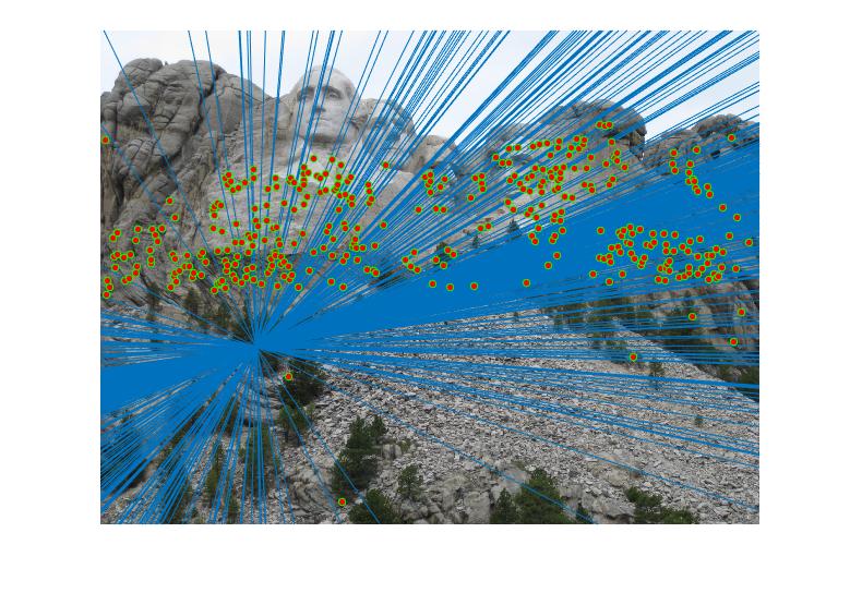
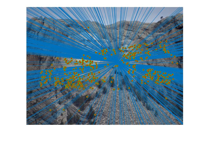
RESULTS 2
|
|
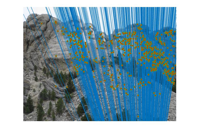
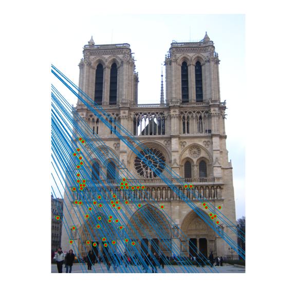
The matching between two images using the SIFT features contains lots of inaccuracies as seen is the project 2. This part of the project aims at reducing the error matching. The brief concept here is that we randomly pick few points from the two images and try to obtain a fundamental matrix using the part 2 of the project. Using this fundamental matrix we try to find number of points that satisfy this fundamental matrix. The points which satisfy this fundamental matrix are called inliers and the ones which do not satisfy are called outliers. The fundamental matrix which satisfy most number of points is the best fundamental matrix for the two images. This algorithm is called RANSAC. In the code the value is fixed to 0.005 which acts as threshold between the inliers and the outliers.
Code for RANSAC
max_iterations = 1000;
[m,n] = size(matches_a);


for iter=1:1:max_iterations
    rand_pos = randsample(m,8);
    rand_samples_a = matches_a(rand_pos,:);
    rand_samples_b = matches_b(rand_pos,:);

    fund_matrix = estimate_fundamental_matrix(rand_samples_a,rand_samples_b);

    for i=1:1:m
        sum(i) = [matches_a(i,1) matches_a(i,2) 1]*fund_matrix*[matches_b(i,1) matches_b(i,2) 1]';
    end
    inliers = find(abs(sum)<0.05);
    if(iter==1)
        max_inliers = inliers;
        min_sum= sum;
        Best_Fmatrix=fund_matrix;
    else
        if(size(inliers,2)>size(max_inliers,2))
            max_inliers = inliers;
            min_sum = sum;
            Best_Fmatrix = fund_matrix;
        end
    end

end
for i=1:1:size(max_inliers,2);
    i
    inliers_a(i,:) = matches_a(max_inliers(1,i),:);
    inliers_b(i,:) = matches_b(max_inliers(1,i),:);
end
RESULTS 3
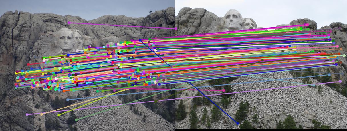
|
We can improve the efficiency of fundamental matrix by normalizing co-ordinates before computing fundamental matrix. We perform the normalization through linear transformations as described below to make the mean of the points zero and the average magnitude about 1.0 or some other small number.
Code for Normalizing Co-ordinates
[xa,ya]=size(Points_a);

ax= Points_a(:,1);
ay= Points_a(:,2);
bx= Points_b(:,1);
by= Points_b(:,2);


mean_ax=mean(ax);
ax_1=ax-(mean_ax*ones(size(ax)));
std_ax=std(ax_1);
istd_ax=1./std_ax;

mean_ay=mean(ay);
ay_1=ay-(mean_ay*ones(size(ay)));
std_ay=std(ay_1);
istd_ay=1./std_ay;


mean_bx=mean(bx);
bx_1=bx-mean_bx*(ones(size(bx)));
std_bx=std(bx_1);
istd_bx=1./std_bx;

mean_by=mean(by);
by_1=by-mean_by*(ones(size(by)));
std_by=std(by_1);
istd_by=1./std_by;


% for u,v
scalingM=[istd_ax,0,0;0,istd_ay,0;0,0,1];
transM=[1,0,-mean_ax; 0,1, -mean_ay; 0,0,1];
one=ones(size(ax));
T=scalingM*transM;   %for first T
mod_ax=T(1,1)*ax+T(1,2)*ay+T(1,3)*one;
mod_ay=T(2,1)*ax+T(2,2)*ay+T(2,3)*one;


% for u1,v1
scalingM1=[istd_bx,0,0;0,istd_by,0;0,0,1];
transM1=[1,0,-mean_bx; 0,1, -mean_by; 0,0,1];
T11=scalingM1*transM1;  %for second T
mod_bx=T11(1,1)*bx+T11(1,2)*by+T11(1,3)*one;
mod_by=T11(2,1)*bx+T11(2,2)*by+T11(2,3)*one;


New_points_a = [mod_ax mod_ay];
New_points_b = [mod_bx mod_by];
 M=[];
%%%%%%%%%%%%%%%%
% Your code here
for i=1:1:xa
    row = [New_points_a(i,1)*New_points_b(i,1) New_points_a(i,1)*New_points_b(i,2) New_points_a(i,1) ...
        New_points_a(i,2)*New_points_b(i,1) New_points_a(i,2)*New_points_b(i,2) New_points_a(i,2) ...
        New_points_b(i,1)  New_points_b(i,2) 1];
    M= [M;row];
end

[U, S, V] = svd(M);
f = V(:, end);
f=f';
F = reshape(f, [3 3]);


[U, S, V] = svd(F);
S(3,3) = 0;
%V = V(:, end);
V=V';
F_matrix1 = U*S*V;


T11=T11';
F_matrix=T11*F_matrix1*T;
F_matrix(isnan(F_matrix))=0;
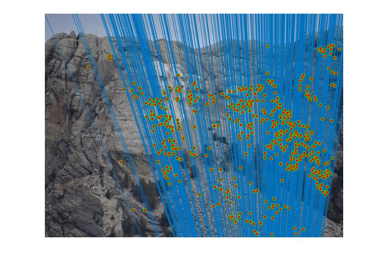
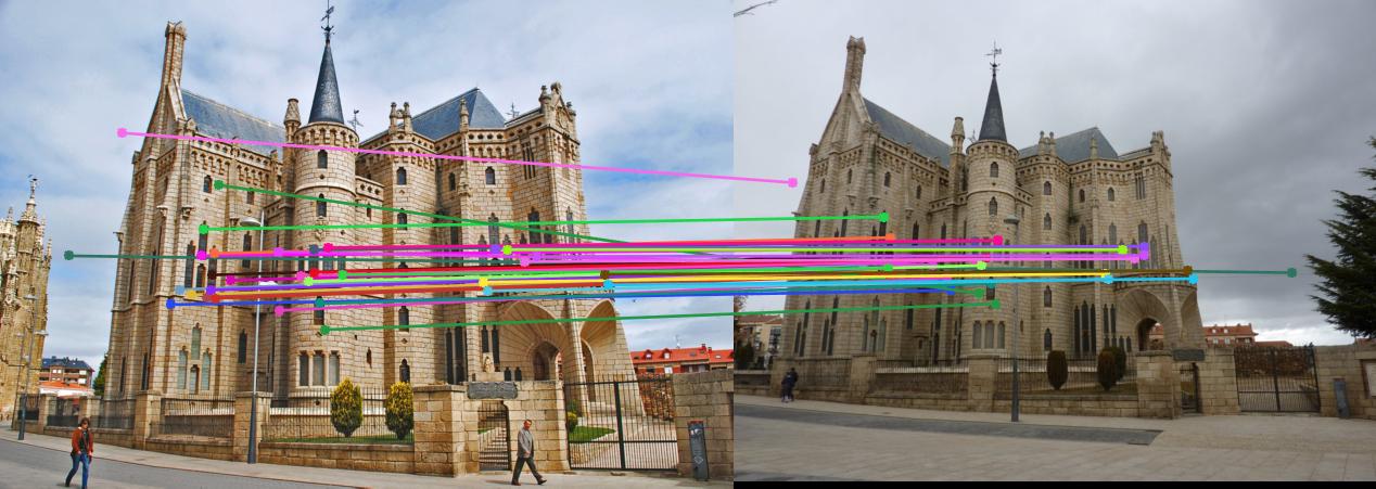
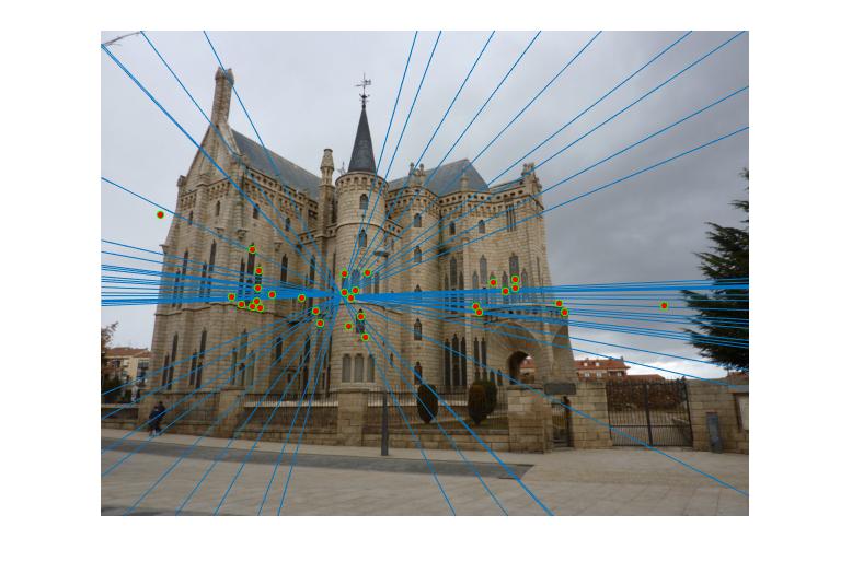
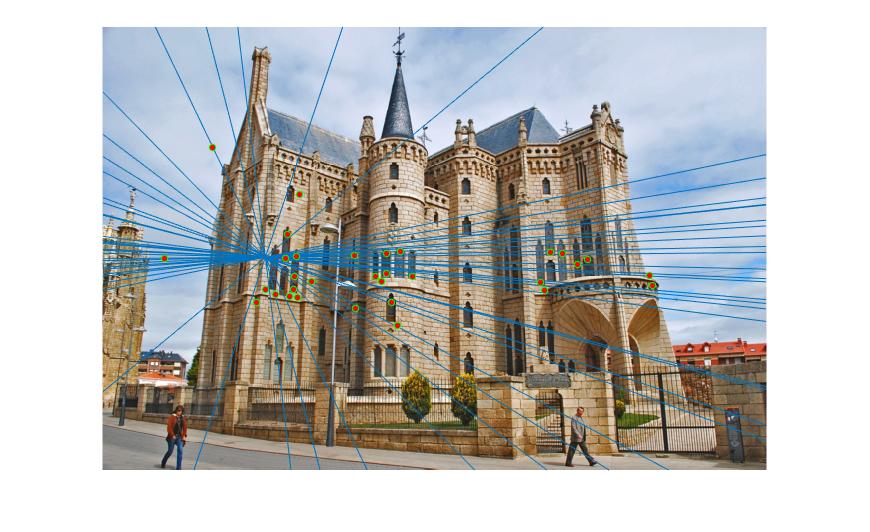
RESULTS 4
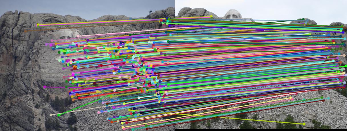
|
As can be clearly seen from result images above, the number of inliers have increased from 125-145 to 500-600 with normalization. The faulty points are reduced by a huge number after normalizing the points.
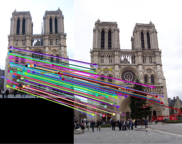
Nortre Dam
|
Episcopal Gaudi
|